Probability-Probability Plots (ligo.skymap.plot.pp)

Axes subclass for making probability–probability (P–P) plots.

Example

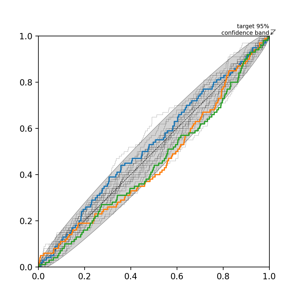
You can create new P–P plot axes by passing the keyword argument projection='pp_plot' when creating new Matplotlib axes.

import ligo.skymap.plot
from matplotlib import pyplot as plt
import numpy as np

n = 100
p_values_1 = np.random.uniform(size=n) # One experiment
p_values_2 = np.random.uniform(size=n) # Another experiment
p_values_3 = np.random.uniform(size=n) # Yet another experiment

fig = plt.figure(figsize=(5, 5))
ax = fig.add_subplot(111, projection='pp_plot')
ax.add_confidence_band(n, alpha=0.95) # Add 95% confidence band
ax.add_diagonal() # Add diagonal line
ax.add_lightning(n, 20) # Add some random realizations of n samples
ax.add_series(p_values_1, p_values_2, p_values_3) # Add our data

(Source code, png, hires.png, pdf)

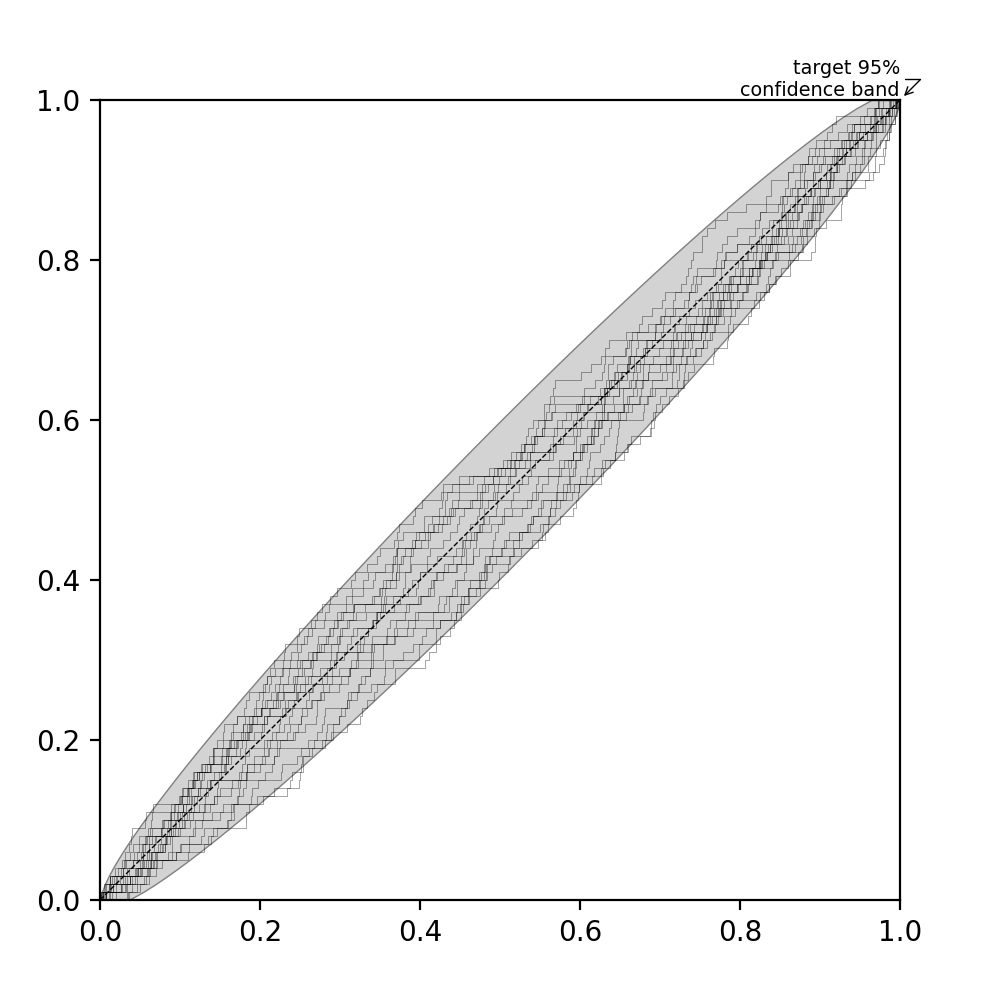
Or, you can call the constructor of PPPlot directly.

from ligo.skymap.plot import PPPlot
from matplotlib import pyplot as plt
import numpy as np

n = 100

rect = [0.1, 0.1, 0.8, 0.8] # Where to place axes in figure
fig = plt.figure(figsize=(5, 5))
ax = PPPlot(fig, rect)
fig.add_axes(ax)
ax.add_confidence_band(n, alpha=0.95)
ax.add_lightning(n, 20)
ax.add_diagonal()

(Source code, png, hires.png, pdf)

class ligo.skymap.plot.pp.PPPlot(*args, **kwargs)

Bases: Axes

Construct a probability–probability (P–P) plot.

Build an Axes in a figure.

Parameters:

figFigure

The Axes is built in the Figure fig.

*args

*args can be a single (left, bottom, width, height) rectangle or a single Bbox. This specifies the rectangle (in figure coordinates) where the Axes is positioned.

*args can also consist of three numbers or a single three-digit number; in the latter case, the digits are considered as independent numbers. The numbers are interpreted as (nrows, ncols, index): (nrows, ncols) specifies the size of an array of subplots, and index is the 1-based index of the subplot being created. Finally, *args can also directly be a SubplotSpec instance.

sharex, shareyAxes, optional

The x- or y-axis is shared with the x- or y-axis in the input Axes.

frameonbool, default: True

Whether the Axes frame is visible.

box_aspectfloat, optional

Set a fixed aspect for the Axes box, i.e. the ratio of height to width. See set_box_aspect for details.

**kwargs

Other optional keyword arguments:

Properties: adjustable: {‘box’, ‘datalim’} agg_filter: a filter function, which takes a (m, n, 3) float array and a dpi value, and returns a (m, n, 3) array and two offsets from the bottom left corner of the image alpha: scalar or None anchor: (float, float) or {‘C’, ‘SW’, ‘S’, ‘SE’, ‘E’, ‘NE’, …} animated: bool aspect: {‘auto’, ‘equal’} or float autoscale_on: bool autoscalex_on: unknown autoscaley_on: unknown axes_locator: Callable[[Axes, Renderer], Bbox] axisbelow: bool or ‘line’ box_aspect: float or None clip_box: BboxBase or None clip_on: bool clip_path: Patch or (Path, Transform) or None facecolor or fc: color figure: Figure frame_on: bool gid: str in_layout: bool label: object mouseover: bool navigate: bool navigate_mode: unknown path_effects: list of AbstractPathEffect picker: None or bool or float or callable position: [left, bottom, width, height] or Bbox prop_cycle: Cycler rasterization_zorder: float or None rasterized: bool sketch_params: (scale: float, length: float, randomness: float) snap: bool or None subplotspec: unknown title: str transform: Transform url: str visible: bool xbound: (lower: float, upper: float) xlabel: str xlim: (left: float, right: float) xmargin: float greater than -0.5 xscale: unknown xticklabels: unknown xticks: unknown ybound: (lower: float, upper: float) ylabel: str ylim: (bottom: float, top: float) ymargin: float greater than -0.5 yscale: unknown yticklabels: unknown yticks: unknown zorder: float

Returns:

Axes

The new Axes object.

add_confidence_band(nsamples, alpha=0.95, annotate=True, **kwargs)

Add a target confidence band.

Parameters:

nsamplesint

Number of P-values

alphafloat, default: 0.95

Confidence level

annotatebool, optional, default: True

If True, then label the confidence band.

Other Parameters:

**kwargs

optional extra arguments to matplotlib.axes.Axes.fill_betweenx

add_diagonal(*args, **kwargs)

Add a diagonal line to the plot, running from (0, 0) to (1, 1).

Other Parameters:

kwargs

optional extra arguments to matplotlib.axes.Axes.plot

add_lightning(nsamples, ntrials, **kwargs)

Add P-values drawn from a random uniform distribution, as a visual representation of the acceptable scatter about the diagonal.

Parameters:

nsamplesint

Number of P-values in each trial

ntrialsint

Number of line series to draw.

Other Parameters:

kwargs

optional extra arguments to matplotlib.axes.Axes.plot

add_series(*p_values, **kwargs)

Add a series of P-values to the plot.

Parameters:

p_valuesnumpy.ndarray

One or more lists of P-values.

If an entry in the list is one-dimensional, then it is interpreted as an unordered list of P-values. The ranked values will be plotted on the horizontal axis, and the cumulative fraction will be plotted on the vertical axis.

If an entry in the list is two-dimensional, then the first subarray is plotted on the horizontal axis and the second subarray is plotted on the vertical axis.

drawstyle{‘steps’, ‘lines’, ‘default’}

Plotting style. If steps, then plot steps to represent a piecewise constant function. If lines, then connect points with straight lines. If default then use steps if there are more than 2 pixels per data point, or else lines.

Other Parameters:

kwargs

optional extra arguments to matplotlib.axes.Axes.plot

add_worst(*p_values)

Mark the point at which the deviation is largest.

Parameters:

p_valuesnumpy.ndarray

Same as in add_series.

set(*, adjustable=<UNSET>, agg_filter=<UNSET>, alpha=<UNSET>, anchor=<UNSET>, animated=<UNSET>, aspect=<UNSET>, autoscale_on=<UNSET>, autoscalex_on=<UNSET>, autoscaley_on=<UNSET>, axes_locator=<UNSET>, axisbelow=<UNSET>, box_aspect=<UNSET>, clip_box=<UNSET>, clip_on=<UNSET>, clip_path=<UNSET>, facecolor=<UNSET>, frame_on=<UNSET>, gid=<UNSET>, in_layout=<UNSET>, label=<UNSET>, mouseover=<UNSET>, navigate=<UNSET>, path_effects=<UNSET>, picker=<UNSET>, position=<UNSET>, prop_cycle=<UNSET>, rasterization_zorder=<UNSET>, rasterized=<UNSET>, sketch_params=<UNSET>, snap=<UNSET>, subplotspec=<UNSET>, title=<UNSET>, transform=<UNSET>, url=<UNSET>, visible=<UNSET>, xbound=<UNSET>, xlabel=<UNSET>, xlim=<UNSET>, xmargin=<UNSET>, xscale=<UNSET>, xticklabels=<UNSET>, xticks=<UNSET>, ybound=<UNSET>, ylabel=<UNSET>, ylim=<UNSET>, ymargin=<UNSET>, yscale=<UNSET>, yticklabels=<UNSET>, yticks=<UNSET>, zorder=<UNSET>)

Set multiple properties at once.

Supported properties are

Properties:

adjustable: {‘box’, ‘datalim’} agg_filter: a filter function, which takes a (m, n, 3) float array and a dpi value, and returns a (m, n, 3) array and two offsets from the bottom left corner of the image alpha: scalar or None anchor: (float, float) or {‘C’, ‘SW’, ‘S’, ‘SE’, ‘E’, ‘NE’, …} animated: bool aspect: {‘auto’, ‘equal’} or float autoscale_on: bool autoscalex_on: unknown autoscaley_on: unknown axes_locator: Callable[[Axes, Renderer], Bbox] axisbelow: bool or ‘line’ box_aspect: float or None clip_box: BboxBase or None clip_on: bool clip_path: Patch or (Path, Transform) or None facecolor or fc: color figure: Figure frame_on: bool gid: str in_layout: bool label: object mouseover: bool navigate: bool navigate_mode: unknown path_effects: list of AbstractPathEffect picker: None or bool or float or callable position: [left, bottom, width, height] or Bbox prop_cycle: Cycler rasterization_zorder: float or None rasterized: bool sketch_params: (scale: float, length: float, randomness: float) snap: bool or None subplotspec: unknown title: str transform: Transform url: str visible: bool xbound: (lower: float, upper: float) xlabel: str xlim: (left: float, right: float) xmargin: float greater than -0.5 xscale: unknown xticklabels: unknown xticks: unknown ybound: (lower: float, upper: float) ylabel: str ylim: (bottom: float, top: float) ymargin: float greater than -0.5 yscale: unknown yticklabels: unknown yticks: unknown zorder: float