stats.inspiral_extrinsics module
The goal of this module is to implement the probability of getting a given set
of extrinsic parameters for a set of detectors parameterized by n-tuples of
trigger parameters: (snr, horizon distance, end time and phase) assuming that
the event is a gravitational wave signal, s, coming from an isotropic
distribution in location, orientation and the volume of space. The
implementation of this in the calling code can be found in
stats.inspiral_lr.
The probabilities are factored in the following way:
where:
See the following for details:
InspiralExtrinsics– helper class to implement the full probability expressionTimePhaseSNR– implementation of term 1 abovep_of_instruments_given_horizons– implementation of term 2 above
and gstlal_inspiral_plot_extrinsic_params for some visualizations of
these PDFs.
Sanity Checks
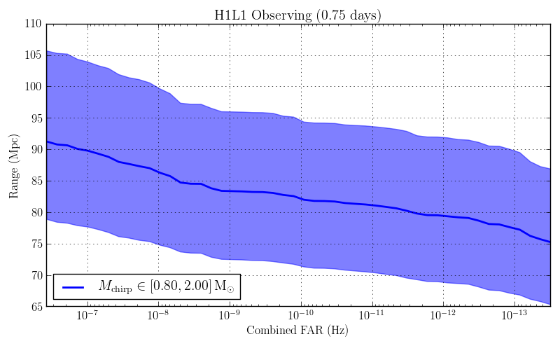
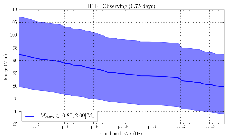
The code here is new for O3. We compared the result to the O2 code on 100,000 seconds of data searching for binary neutron stars in H and L. The injection set was identical. Although an improvement for an HL search was not expected, in fact it appears that the reimplementation is a bit more sensitive.
O2 Code |
O3 Code |
|
|---|---|---|
Found/Missed |
939 / 2270 |
951 / 2258 |
Range |
|
|
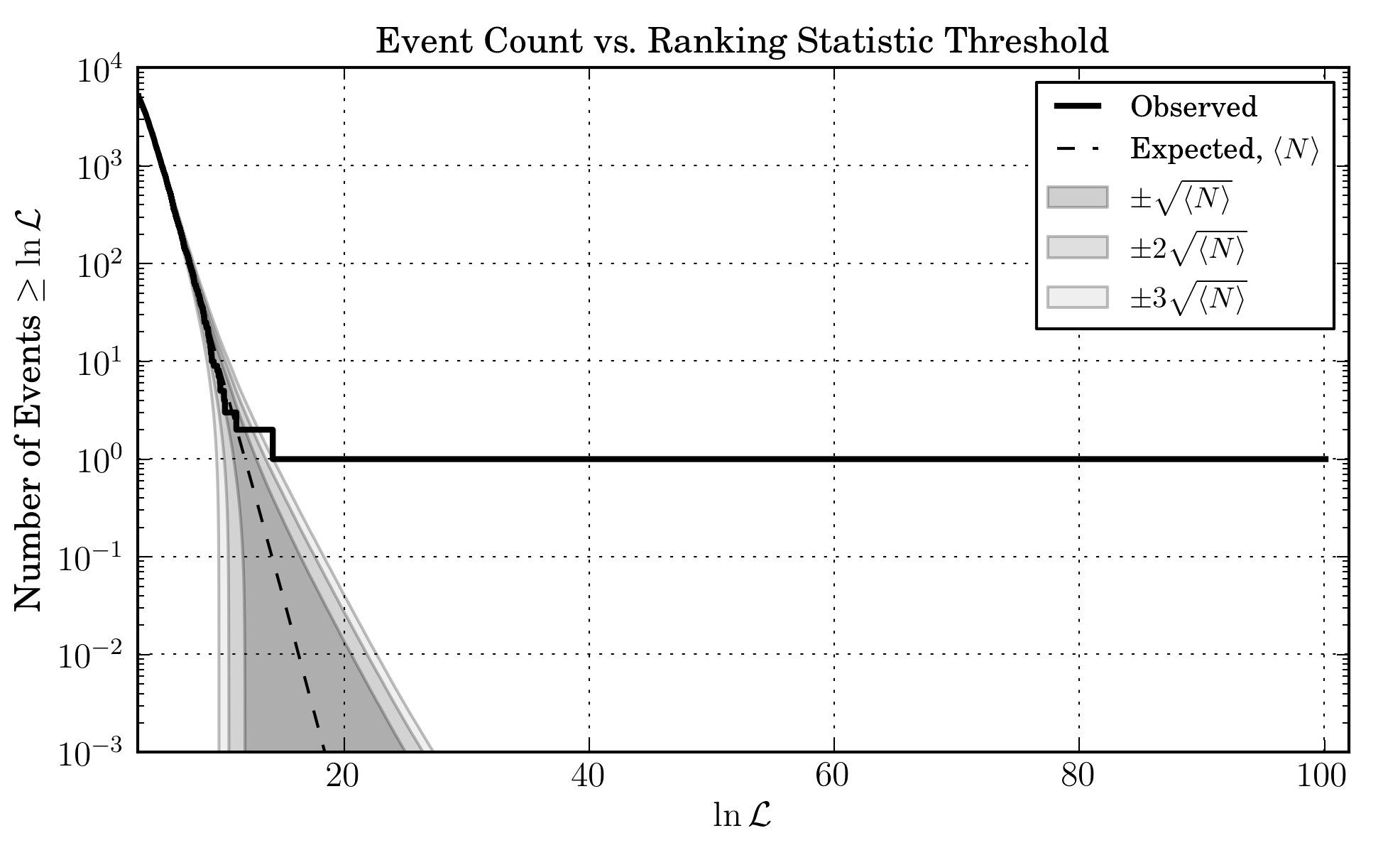
Count vs LR |
|
|

Double vs triple found injections
In this check we ran two analyses:
An HL only analysis
An HLV analysis
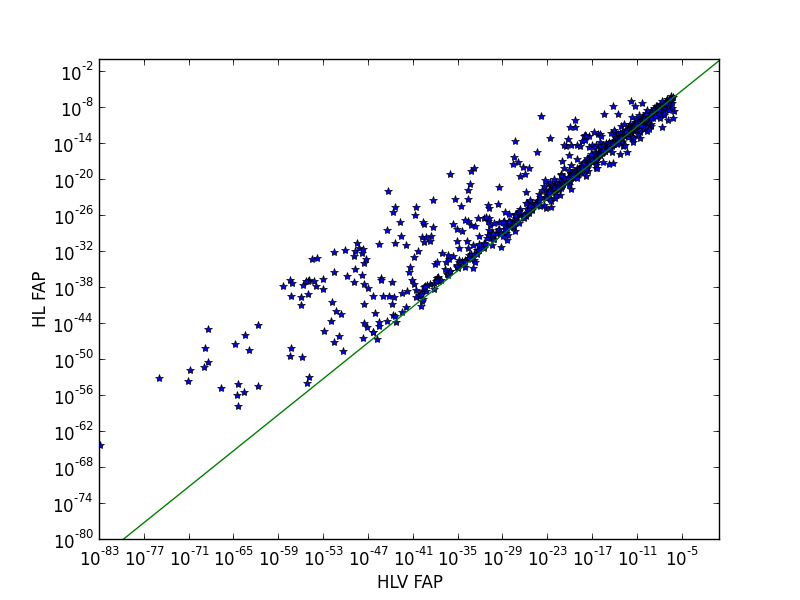
Both were over the same time period. A common set of found injections was identified and the false alarm probability (FAP) was computed for the doubles and triples. Ideally false alarm probabilities for all doubles would be higher than all triples, but this is not a requirement since noise and especially glitches can cause a triple to be ranked below a double. The plot below shows that at least the trend is correct. NOTE we are not currently computing doubles and triples and picking the best.
Check of PDFs
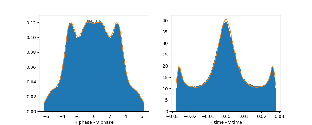
We tested the procedure for evaluating the probabilility using the procedure described below (orange) against a monte carlo (blue). The details are in this script
https://git.ligo.org/lscsoft/gstlal/blob/master/gstlal-inspiral/tests/dtdphitest.py
You can modify this source code to implement different checks. The one implemented is to plot the marginal distributions of time delay and phase delay between Hanford and Virgo under the condition that the measured effective distance is the same. NOTE this test assumes the same covariance matrix for noise as the code below in order to test the procedure, but it doesn’t prove that the assumption is optimal.
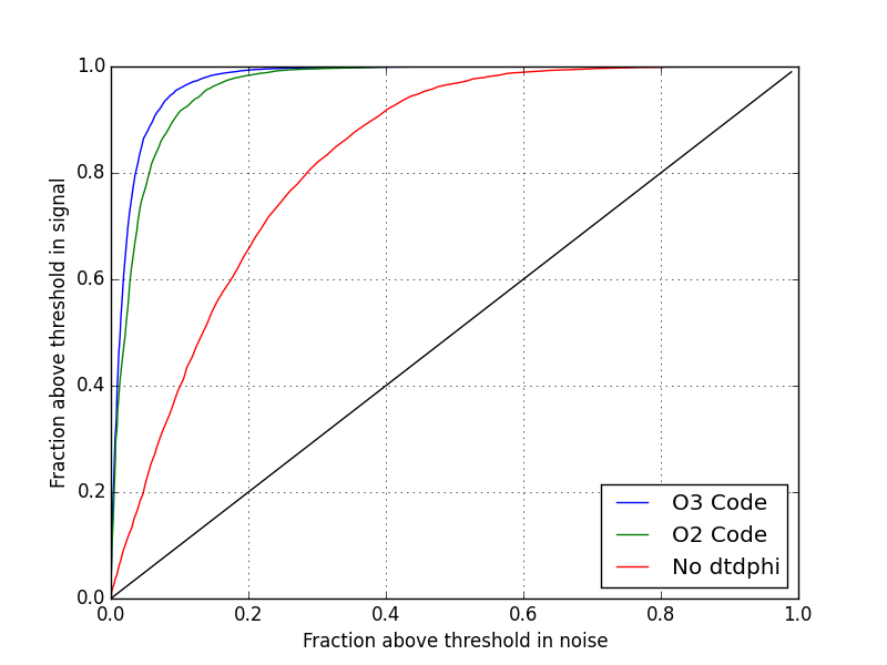
ROC Curves for HL Analysis with the O2 and O3 code
Using the code here
we generated ROC curves for discriminiting a synthetic signal and noise model in H and L. Three traces are shown. First, the the SNR only terms in the likelihood ratio, which was the situation in O1 Code (red). Second, the O2 code with the previous implementation of additional dt and dphi terms (green) and finally the current implementation (blue). The improvement of the present implementation is consistent with the above injection results and this further demonstrates that the reimplementation has “done no harm” to the O2 configuration.
Review Status
Do no harm check of O2 results (Complete)
Comparing runs before and after (done)
Checking the probabilities returned by new code and old code to show consistent results (done)
Check of error assumptions (For O3)
Calculate theoretical delta T, delta phi and snr ratio values of an O2 injection set. Then compute same parameters from injections. The difference between those (in e.g., a scatter plot) should give a sense of the errors on those parameters caused by noise. (sarah is working on it)
Eventually use the fisher matrix for the error estimates (chad will do it, but not for O2)
Inclusion of virgo (Partially complete, rest for O3)
Virgo should not make the analysis worse in an average sense. (done, see https://dcc.ligo.org/LIGO-G1801491)
Understand cases where / if virgo does downrank a trigger (addressed by below)
Consider having the likelihood calculation maximize over all trigger subsets (Chad and Kipp will do this for O3)
Names |
Hash |
Date |
|---|---|---|
– |
– |
– |
Documentation of classes and functions
- class stats.inspiral_extrinsics.InspiralExtrinsics(instruments=('H1', 'K1', 'L1', 'V1'), min_instruments=1, filename=None)[source]
Bases:
objectHelper class to use preinitialized data for the extrinsic parameter calculation. Presently only H,L,V is supported. K could be added by making new data files with
TimePhaseSNRandp_of_instruments_given_horizons.This class is used to compute p_of_instruments_given_horizons and the probability of getting time phase and snrs from a given instrument combination. The argument min_instruments will be used to normalize the p_of_instruments_given_horizons to set the probability of a combination with fewer than min_instruments to be 0.
>>> IE = InspiralExtrinsics()
>>> IE.p_of_instruments_given_horizons(("H1","L1"), {"H1":200, "L1":200})
0.36681567679586446
>>> IE.p_of_instruments_given_horizons(("H1","L1"), {"H1":20, "L1":200})
0.0021601523270060085
>>> IE.p_of_instruments_given_horizons(("H1","L1"), {"H1":200, "L1":200, "V1":200})
0.14534898937680402
>>> IE.p_of_instruments_given_horizons(("H1","L1"), {"H1":200, "L1":200, "V1":200}) + IE.p_of_instruments_given_horizons(("H1","V1"), {"H1":200, "L1":200, "V1":200}) + IE.p_of_instruments_given_horizons(("L1","V1"), {"H1":200, "L1":200, "V1":200}) + IE.p_of_instruments_given_horizons(("H1","L1","V1"), {"H1":200, "L1":200, "V1":200})
1.0
>>> IE.time_phase_snr({"H1":0.001, "L1":0.0, "V1":0.004}, {"H1":1.3, "L1":4.6, "V1":5.3}, {"H1":20, "L1":20, "V1":4}, {"H1":200, "L1":200, "V1":50})
array([  1.01240596e-06], dtype=float32)
>>> IE.time_phase_snr({"H1":0.001, "L1":0.0, "V1":0.004}, {"H1":1.3, "L1":1.6, "V1":5.3}, {"H1":20, "L1":20, "V1":4}, {"H1":200, "L1":200, "V1":50})
array([  1.47201028e-15], dtype=float32)
The total probability would be the product, e.g.,
>>> IE.time_phase_snr({"H1":0.001, "L1":0.0, "V1":0.004}, {"H1":1.3, "L1":4.6, "V1":5.3}, {"H1":20, "L1":20, "V1":8}, {"H1":200, "L1":200, "V1":200}) * IE.p_of_instruments_given_horizons(("H1","L1","V1"), {"H1":200, "L1":200, "V1":200})
array([  2.00510986e-08], dtype=float32)
See the following for more details:
- p_of_ifos = {('H1', 'K1'): <stats.inspiral_extrinsics.p_of_instruments_given_horizons object>, ('H1', 'K1', 'L1'): <stats.inspiral_extrinsics.p_of_instruments_given_horizons object>, ('H1', 'K1', 'L1', 'V1'): <stats.inspiral_extrinsics.p_of_instruments_given_horizons object>, ('H1', 'K1', 'V1'): <stats.inspiral_extrinsics.p_of_instruments_given_horizons object>, ('H1', 'L1'): <stats.inspiral_extrinsics.p_of_instruments_given_horizons object>, ('H1', 'L1', 'V1'): <stats.inspiral_extrinsics.p_of_instruments_given_horizons object>, ('H1', 'V1'): <stats.inspiral_extrinsics.p_of_instruments_given_horizons object>, ('K1', 'L1'): <stats.inspiral_extrinsics.p_of_instruments_given_horizons object>, ('K1', 'L1', 'V1'): <stats.inspiral_extrinsics.p_of_instruments_given_horizons object>, ('K1', 'V1'): <stats.inspiral_extrinsics.p_of_instruments_given_horizons object>, ('L1', 'V1'): <stats.inspiral_extrinsics.p_of_instruments_given_horizons object>}
- time_phase_snr = None
- class stats.inspiral_extrinsics.TimePhaseSNR(instruments=('H1', 'L1', 'V1', 'K1'), transtt=None, transtp=None, transpt=None, transpp=None, transdd=None, norm=None, tree_data=None, margsky=None, verbose=False, margstart=0, margstop=None, SNR=None, psd_fname=None, NSIDE=16, n_inc_angle=33, n_pol_angle=33)[source]
Bases:
objectThe goal of this is to compute:
Instead of evaluating the above probability we will parameterize it by pulling out an overall term that scales as the network SNR to the negative fourth power.
We reduce the dimensionality by computing things relative to the first instrument in alphabetical order and use effective distance instead of SNR, e.g.,
where now the absolute geocenter end time or coalescence phase does not matter since our new variables are relative to the first instrument in alphabetical order (denoted with 0 subscript). Since the first component of each of the new vectors is one by construction we don’t track it and have reduced the dimensionality by three.
We won’t necessarily evalute exactly this distribution, but something that should be proportional to it. In order to evaluate this distribution. We assert that physical signals have a uniform distribution in earth based coordinates,
where
Then we assert that:
Where by construction
Where
The geometric interpretation is shown in the following figure:
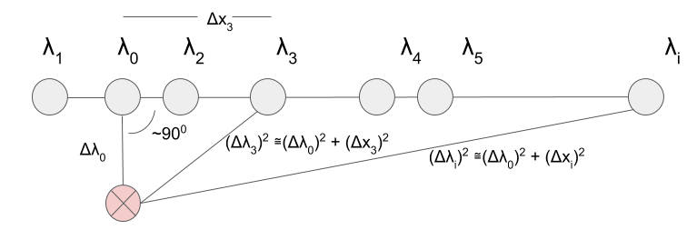
In order for this endeavor to be successful, we still need a fast way to find the nearest neighbor. We use scipy KDTree to accomplish this.
- property combos
return instrument combos for all the instruments internally stored in self.responses
>>> TimePhaseSNR.combos
(('H1', 'L1'), ('H1', 'L1', 'V1'), ('H1', 'V1'), ('L1', 'V1'))
- dtdphideffpoints(time, phase, deff, slices)[source]
Given a dictionary of time, phase and deff, which could be lists of values, pack the delta t delta phi and eff distance ratios transformed by the covariance matrix according to the rules provided by slices.
>>> TimePhaseSNR.dtdphideffpoints({"H1":0, "L1":-.001, "V1":.001}, {"H1":0, "L1":0, "V1":1}, {"H1":1, "L1":3, "V1":4}, TimePhaseSNR.slices)
array([[ 1.        ,  0.        , -5.        , -1.        , -2.54647899,
        -5.        , -2.        , -2.54647899, -5.        ]], dtype=float32)
NOTE You must have the same ifos in slices as in the time, phase, deff dictionaries. The result of self.slices gives slices for all the instruments stored in self.responses
- classmethod from_hdf5(fname, other_fnames=[], instruments=('H1', 'K1', 'L1', 'V1'), **kwargs)[source]
Initialize one of these from a file instead of computing it from scratch
- classmethod instrument_combos(instruments, min_instruments=2)[source]
Given a list of instrument produce all the possible combinations of min_instruents or greater, e.g.,
>>> TimePhaseSNR.instrument_combos(("H1","V1","L1"), min_instruments = 3)
(('H1', 'L1', 'V1'),)
>>> TimePhaseSNR.instrument_combos(("H1","V1","L1"), min_instruments = 2)
(('H1', 'L1'), ('H1', 'L1', 'V1'), ('H1', 'V1'), ('L1', 'V1'))
>>> TimePhaseSNR.instrument_combos(("H1","V1","L1"), min_instruments = 1)
(('H1',), ('H1', 'L1'), ('H1', 'L1', 'V1'), ('H1', 'V1'), ('L1',), ('L1', 'V1'), ('V1',))
NOTE: these combos are always returned in alphabetical order
- instrument_pair_slices(pairs)[source]
define slices into tree data for a given set of instrument pairs (which is possibly a subset of the full availalbe pairs)
- instrument_pairs(instruments)[source]
Given a list of instruments, construct all possible pairs
>>> TimePhaseSNR.instrument_pairs(("H1","K1","V1","L1"))
(('H1', 'K1'), ('H1', 'L1'), ('H1', 'V1'))
NOTE: These are always in alphabetical order
- locations = {'H1': array([-2161414.92636, -3834695.17889, 4600350.22664]), 'K1': array([-3777336.024, 3484898.411, 3765313.697]), 'L1': array([ -74276.0447238, -5496283.71971 , 3224257.01744 ]), 'V1': array([4546374.099 , 842989.697626, 4378576.96241 ])}
- numchunks = 20
- property pairs
Return all possible pairs of instruments for the instruments internally stored in self.responses >>> TimePhaseSNR.pairs ((‘H1’, ‘L1’), (‘H1’, ‘V1’), (‘L1’, ‘V1’))
- responses = {'H1': array([[-0.3926141 , -0.07761341, -0.24738905], [-0.07761341, 0.31952408, 0.22799784], [-0.24738905, 0.22799784, 0.07309003]], dtype=float32), 'K1': array([[-0.18598965, 0.1531668 , -0.32495147], [ 0.1531668 , 0.3495183 , -0.1708744 ], [-0.32495147, -0.1708744 , -0.16352864]], dtype=float32), 'L1': array([[ 0.41128087, 0.14021027, 0.24729459], [ 0.14021027, -0.10900569, -0.18161564], [ 0.24729459, -0.18161564, -0.30227515]], dtype=float32), 'V1': array([[ 0.24387404, -0.09908378, -0.23257622], [-0.09908378, -0.44782585, 0.1878331 ], [-0.23257622, 0.1878331 , 0.2039518 ]], dtype=float32)}
- property slices
This provides a way to index into the internal tree data for the delta T, delta phi, and deff ratios for each instrument pair.
>>> TimePhaseSNR.slices
{('H1', 'L1'): [0, 1, 2], ('H1', 'V1'): [3, 4, 5], ('L1', 'V1'): [6, 7, 8]}
- classmethod tile(NSIDE=16, n_inc_angle=33, n_pol_angle=33, verbose=False)[source]
Tile the sky with equal area tiles defined by the healpix NSIDE parameter for sky pixels. Also tile polarization uniformly and inclination uniform in cosine with n_inc_angle and n_pol_angle. Convert these sky coordinates to time, phase and deff for each instrument in self.responses. Return the sky tiles in the detector coordinates as dictionaries. The default values have millions of points in the 4D grid
- stats.inspiral_extrinsics.chunker(seq, size, start=None, stop=None)[source]
A generator to break up a sequence into chunks of length size, plus the remainder, e.g.,
>>> for x in chunker([1, 2, 3, 4, 5, 6, 7], 3):
...     print x
...
[1, 2, 3]
[4, 5, 6]
[7]
- stats.inspiral_extrinsics.margprob(Dmat)[source]
Compute the marginalized probability along the second dimension of a matrix Dmat. Assumes the probability is the form exp(-x_i^2/2.)
>>> margprob(numpy.array([[1.,2.,3.,4.], [2.,3.,4.,5.]]))
[0.41150885406464954, 0.068789418217400547]
- class stats.inspiral_extrinsics.p_of_instruments_given_horizons(instruments=('H1', 'L1', 'V1'), snr_thresh=4.0, nbins=41, hmin=0.05, hmax=20.0, histograms=None, bin_start=0, bin_stop=None)[source]
Bases:
objectThe goal of this class is to compute
where
with
TimePhaseSNR. We add a random jitter to each SNR according to a chi-squared distribution with two degrees of freedom.The result of this is stored in a histogram, which means we choose quanta of horizon distances to do the calculation. Since we only care about the ratios of horizon distances in this calculation, the horizon distance for the first detector in alphabetical order are by convention 1. The ratios of horizon distances for the other detectors are logarithmically spaced between 0.05 and 20. Below are a couple of example histograms.
Example: 1D histogram for
This is a 1x41 array representing the following probabilities:
…
…
Note, linear interpolation is used over the bins
Example 2D histogram for
This is a 41x41 array representing the following probabilities:
…
…
…
…
…
…
…
…
…
…
Note, linear interpolation is used over the bins