Generating waveforms
Through pesummary’s SamplesDict class, we can easily
generate a waveform based on a specific set of posterior samples either in the
time domain or the frequency domain. This is through the td_waveform and
fd_waveform methods. Below we show an example using the publically available
GW190814 posterior samples.
First let us plot a waveform in the time domain,
 1from pesummary.gw.fetch import fetch_open_samples
 2import matplotlib.pyplot as plt
 3
 4# First we download and read the publically available posterior samples
 5f = fetch_open_samples("GW190814", unpack=True, path="GW190814.h5")
 6samples = f.samples_dict
 7EOB = samples["C01:SEOBNRv4PHM"]
 8
 9# Next we generate the plus and cross polarizations in the time domain for the
10# maximum likelihood sample
11approximant = "SEOBNRv4PHM"
12delta_t = 1. / 4096
13f_low = 20.
14wvfs = EOB.maxL_td_waveform(approximant, delta_t, f_low, f_ref=f_low)
15
16# Alternatively, we may generate the plus and cross polarizations in the time
17# domain for a specific sample with the ind kwarg
18ind = 100
19wvfs = EOB.td_waveform(approximant, delta_t, f_low, f_ref=f_low, ind=ind)
20
21# It is often useful to know what the strain is at a given gravitational wave
22# detector. This involves calculating the antenna response function. If we
23# wanted to generate the maximum likelihood strain projected onto the LIGO
24# Livingtson detector, we may simply run
25ht = EOB.maxL_td_waveform(approximant, delta_t, f_low, f_ref=f_low, project="L1")
26
27# In all cases, a `gwpy.timeseries.TimeSeries` object is returned. This can
28# therefore easily be plotted with
29fig = plt.figure()
30plt.plot(ht.times, ht)
31plt.savefig("GW190814_SEOBNRv4PHM_td.png")

In the above example only the maximum likelihood waveform is plotted. Sometimes
it is useful to know the uncertainty on this waveform. We can calculate and plot
the 1 sigma and 2 sigma symmetric confidence intervals of this waveform by
taking advantage of the level kwarg,
 1from pesummary.gw.fetch import fetch_open_samples
 2import matplotlib.pyplot as plt
 3
 4f = fetch_open_samples("GW190814", unpack=True, path="GW190814.h5")
 5samples = f.samples_dict
 6EOB = samples["C01:SEOBNRv4PHM"]
 7_ = EOB.downsample(1000)
 8approximant = "SEOBNRv4PHM"
 9delta_t = 1. / 4096
10f_low = 20.
11ht, upper, lower, bound_times = EOB.maxL_td_waveform(
12    approximant, delta_t, f_low, f_ref=f_low, project="L1", level=[0.68, 0.95],
13    multi_process=4
14)
15fig = plt.figure()
16plt.plot(ht.times, ht)
17plt.fill_between(bound_times, upper[0], lower[0], color='r', alpha=0.4)
18plt.fill_between(bound_times, upper[1], lower[1], color='r', alpha=0.2)
19plt.xlim(1249852257.01 - 0.1, 1249852257.01 + 0.04)
20plt.savefig("GW190814_SEOBNRv4PHM_td_with_uncertainty.png")
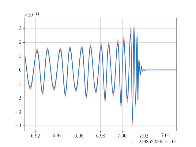
Here we have chosen to downsample the posterior samples to 1000 samples
(_ = EOB.downsample(1000)) and used 4 CPUs (multi_process=4)
to speed up waveform generation.
We can also generate a waveform in the frequency domain with,
 1from pesummary.gw.fetch import fetch_open_samples
 2import matplotlib.pyplot as plt
 3
 4# First we download and read the publically available posterior samples
 5f = fetch_open_samples(
 6    "GW190814", catalog="GWTC-2", unpack=True, path="GW190814.h5"
 7)
 8samples = f.samples_dict
 9Phenom = samples["C01:IMRPhenomPv3HM"]
10
11# Next we generate the plus and cross polarizations in the frequency domain for
12# the maximum likelihood sample
13approximant = "IMRPhenomPv3HM"
14delta_f = 1. / 256
15f_low = 20.
16f_high = 1024.
17wvfs = Phenom.maxL_fd_waveform(approximant, delta_f, f_low, f_high, f_ref=f_low)
18
19# Alternatively, we may generate the plus and cross polarizations in the
20# frequency domain for a specific sample with the ind kwarg
21ind = 100
22wvfs = Phenom.fd_waveform(approximant, delta_f, f_low, f_high, f_ref=f_low, ind=ind)
23
24# It is often useful to know what the strain is at a given gravitational wave
25# detector. This involves calculating the antenna response function. If we
26# wanted to generate the maximum likelihood strain projected onto the LIGO
27# Livingtson detector, we may simply run
28ht = Phenom.maxL_fd_waveform(approximant, delta_f, f_low, f_high, f_ref=f_low, project="L1")
29
30# In all cases, a `gwpy.frequencyseries.FrequencySeries` object is returned.
31# This can therefore easily be plotted with
32fig = plt.figure()
33plt.plot(ht.frequencies, ht)
34plt.savefig("GW190814_IMRPhenomPv3HM_fd.png")
For more details about the waveform generator in pesummary see,
- pesummary.gw.waveform.fd_waveform(samples, approximant, delta_f, f_low, f_high, f_ref=20.0, project=None, ind=0, longAscNodes=0.0, eccentricity=0.0, LAL_parameters=None, mode_array=None, pycbc=False, flen=None, flags={}, debug=False, **kwargs)[source]
Generate a gravitational wave in the frequency domain
- Parameters:
approximant (str) – name of the approximant to use when generating the waveform
delta_f (float) – spacing between frequency samples
f_low (float) – frequency to start evaluating the waveform
f_high (float) – frequency to stop evaluating the waveform
f_ref (float, optional) – reference frequency
project (str, optional) – name of the detector to project the waveform onto. If None, the plus and cross polarizations are returned. Default None
ind (int, optional) – index for the sample you wish to plot
longAscNodes (float, optional) – longitude of ascending nodes, degenerate with the polarization angle. Default 0.
eccentricity (float, optional) – eccentricity at reference frequency. Default 0.
LAL_parameters (LALDict, optional) – LAL dictionary containing accessory parameters. Default None
mode_array (2d list) – 2d list of modes you wish to include in waveform. Must be of the form [[l1, m1], [l2, m2]]
pycbc (Bool, optional) – return a the waveform as a pycbc.frequencyseries.FrequencySeries object
flen (int) – Length of the frequency series in samples. Default is None. Only used when pycbc=True
debug (bool, optional) – if True, return the model object used to generate the waveform. Only used when the waveform approximant is not in LALSimulation
flags (dict, optional) – waveform specific flags to add to LAL dictionary
**kwargs (dict, optional) – all kwargs passed to _calculate_hp_hc_fd
- pesummary.gw.waveform.td_waveform(samples, approximant, delta_t, f_low, f_ref=20.0, project=None, ind=0, longAscNodes=0.0, eccentricity=0.0, LAL_parameters=None, mode_array=None, pycbc=False, level=None, multi_process=1, flags={}, debug=False, **kwargs)[source]
Generate a gravitational wave in the time domain
- Parameters:
approximant (str) – name of the approximant to use when generating the waveform
delta_t (float) – spacing between frequency samples
f_low (float) – frequency to start evaluating the waveform
f_ref (float, optional) – reference frequency
project (str, optional) – name of the detector to project the waveform onto. If None, the plus and cross polarizations are returned. Default None
ind (int, optional) – index for the sample you wish to plot
longAscNodes (float, optional) – longitude of ascending nodes, degenerate with the polarization angle. Default 0.
eccentricity (float, optional) – eccentricity at reference frequency. Default 0.
LAL_parameters (LALDict, optional) – LAL dictionary containing accessory parameters. Default None
mode_array (2d list) – 2d list of modes you wish to include in waveform. Must be of the form [[l1, m1], [l2, m2]]
pycbc (Bool, optional) – return a the waveform as a pycbc.timeseries.TimeSeries object
level (list, optional) – the symmetric confidence interval of the time domain waveform. Level must be greater than 0 and less than 1
multi_process (int, optional) – number of cores to run on when generating waveforms. Only used when level is not None,
flags (dict, optional) – waveform specific flags to add to LAL dictionary. Default {}
kwargs (dict, optional) – all kwargs passed to _td_waveform