|
LALApps 10.1.0.1-da3b9d3
|


|
|
LALApps 10.1.0.1-da3b9d3
|
|

\[ \DeclareMathOperator{\order}{O} \newcommand{\Msol}{{M_{\Sol}}} \newcommand{\Sol}{\odot} \newcommand{\aye}{\mathrm{i}} \newcommand{\conj}[1]{#1^{*}} \newcommand{\diff}{\,\mathrm{d}} \newcommand{\ee}{\mathrm{e}} \newcommand{\magnitude}[1]{\left|#1\right|} \newcommand{\mean}[1]{\left\langle#1\right\rangle} \]
The excess power pipeline implements an "incoherent" search for unmodeled gravitational waves. A schematic diagram of the data flow through the pipeline is shown in this figure.

Here and in what follows we'll discuss the multi-detector version of the pipeline. The pipeline can analyze any number of detectors, but in the 1 detector case much of the pipeline (e.g., the coincidence stages) reduces to no-ops and is uninteresting.
The pipeline begins by scanning the outputs of the gravitational wave detectors for statistically significant excursions from the background noise. In particular, it searches for excursions from the noise, or bursts, that can be characterized by a frequency band and time interval. The raw events identified in the outputs of the individual detectors are clustered, which reduces the event rate and assists in parameter estimation. The clusters are tested for coincidence across instruments, that is events are discarded unless matching events are also found in all other detectors. A set of events that, together, passes the coincidence test will be refered to as a coincident \(n\)-tuple.
Prior to applying the coincidence test, optional delays can be applied to the events. In the LIGO-only case, delays are only applied to events from the L1 detector. The delay facility is used to collect two populations of coincident \(n\)-tuples: \(n\)-tuples with delays applied which are refered to as time-slide coincidences, and \(n\)-tuples with no delays applied which are refered to as zero-lag coincidences.
It is also possible to insert software injections into the detector time series. The injection facility is used to simulate the presense of gravitational waves in the data. When software injections are inserted into the time series, the coincidence test is followed by an injection identification step. This stage identifies two populations of recovered injections: injections that are recovered very well, and injections that are recovered poorly.
The time-slide non-injection \(n\)-tuples, and the \(n\)-tuples corresponding to well-recovered software injections are collected together and their parameters measured to yield two distribution density functions. The parameter distribution density function measured from the time-slide \(n\)-tuples is interpreted as the parameter distribution for noise-like \(n\)-tuples, while the parameter distribution density function measured from the software injections is interpreted as the parameter distribution for gravitational wave-like \(n\)-tuples. The ratio of these two distributions is used to assign a likelihood ratio to each \(n\)-tuple.
Finally, a likelihood-ratio based threshold is applied to each \(n\)-tuple. The zero-lag \(n\)-tuples that survive this final cut are gravitational wave detection candidates. The same cut is applied to software injection \(n\)-tuples to measure the detection efficiency of the pipeline. If the final threshold is adjusted so that just exactly 0 zero-lag \(n\)-tuples survive, the efficiency measured for the pipeline in that configuration can be used to derive an upper-limit result.
lalapps_power — apply excess power event selection algorithm to real or simulated gravitational wave detector data.
lalapps_power –bandwidth Hz [–calibration-cache cache file] –channel-name string –confidence-threshold threshold [–dump-diagnostics XML filename] –filter-corruption samples –frame-cache cache file [–gaussian-noise-rms RMS] –gps-end-time seconds –gps-start-time seconds [–help] –high-pass Hz [–injection-file file name] –low-freq-cutoff Hz [–max-event-rate Hz] –max-tile-bandwidth Hz –max-tile-duration seconds [–mdc-cache cache file] [–mdc-channel channel name] [–output file name] –psd-average-points samples [–ram-limit MebiBytes] –resample-rate Hz [–sim-cache cache file] [–sim-seconds sec.s] [–siminjection-file injection file] [–seed seed] –target-sample-rate Hz –tile-stride-fraction fraction [–user-tag comment] –window-length samples
lalapps_power performs an excess power analysis on real or simulated data. This program's input consists of gravitational wave detector time series data, and an optional list of injections to add to the time series prior to analysis. The program's output is a list of events identified as being statistically significant in the input time series.
Gravitational wave detector time series data is read from LIGO/VIRGO .gwf frame files. This program analyzes data from only a single detector at a time, but it can analyze data that spans multiple frame files. Usually a collection of frame files is specified by providing as input to this program a LAL cache file, as might be obtained from LSCdataFind. Internally, all processing is performed using double-precision IEEE floating point arithmetic. The type of data in the input channel is auto-detected and the data is cast to double precision if needed.
If software injections are desired, then a LIGO_LW XML file containing a sim_burst table describing the software injections must also be provided as input. In the past it has also been possible to read sim_inspiral tables and MDC injection frame files, but these facilities have not been tested in a long time. See the lalapps_binj program described in binj.c for information on constructing injection description files.
The output is written to a LIGO_LW XML file containing a sngl_burst table listing the events found in the input time series. The output file also contains process, process_params, and search_summary tables containing metadata describing the analysis that was performed. In particular, these other tables provide precise information about the instrument and interval of time that the program analyzed.
By default, the output file is named following the standard frame file naming convention.
For example, if a search was run on the Hanford 4 km interferometer and generated triggers starting at GPS time 731488397 s, the triggers cover 33 s after that time, and the command line includes the option "<tt>--comment</tt> TEST", then the file name would be
The output file name can be set explicitly with the –output command line option. If the name ends in ".gz", then it will be gzip-compressed.
–bandwidth HzSet the bandwidth in which the search is to be performed. This must be an integer power of 2. This and the –low-freq-cutoff option together set the frequency band to be searched.
–calibration-cache cache fileSpecify the location of calibration information. cache file gives the path to a LAL-format frame cache file describing locations of .gwf frame files that provide the calibration data ( \(\alpha\) and \(\beta\) coefficients) for the analysis. Frame cache files are explained in the "framedata" package in LAL. This option also controls the units assumed for the data (frame files don't provide that information). When this command line option is present the input time series data is assumed to have units of "ADC counts", otherwise it is assumed to have units of strain.
–channel-name stringSet the name of the data channel to analyze to string. This must match the name of one of the data channels in the input frame files. For example, "<tt>H2:LSC-AS_Q</tt>".
–confidence-threshold thresholdSet the confidence threshold below which events should be discarded. The "confidence" of an event is \(-\ln P(\text{event} | \text{stationary Gaussian white noise})\), so an event with a confidence of 30 has a probability of \(\ee^{-30}\) of having been found in stationary Gaussian white noise. For the LIGO instruments, a practical treshold is typically around 10.
–dump-diagnostics XML filenameDump diagnostic snapshots of internal time and frequency series data to a LIGO Light Weight XML file of the given name. The file is overwritten.
–filter-corruption samplesThe input time series data is passed through a conditioning filter prior to analysis. Generally, the conditioning filter should be expected to corrupt some amount of the beginning and end of the time series due to edge effects. This parameter tells the code how much data, in samples, should be ignored from the start and end of the time series. A reasonable value is 0.5 seconds worth of data.
–frame-cache cache fileObtain the locations of input .gwf frame files from the LAL frame cache file cache file. LAL frame cache files are explained in the "framedata" package in LAL and can be constructed by running LSCDataFind on some systems. One of –frame-cache, or –gaussian-noise-rms must be specified.
–gaussian-noise-rms RMSIf this parameter is provided instead of –frame-cache, then Gaussian white noise will be synthesized and used as the input data. One of –frame-cache, or –gaussian-noise-rms must be specified.
–gps-end-time secondsSet the GPS time up to which input data should be read. Non-integer values are permitted, but the fractional part must not contain more than 9 digits (accurate to nanoseconds).
–gps-start-time secondsSet the GPS time from which to start reading input data. Non-integer values are permitted, but the fractional part must not contain more than 9 digits (accurate to nanoseconds).
–helpDisplay a usage message and exit.
–high-pass HzThe input time series is high-pass filtered as part of the input data conditioning. This argument sets the cut-off frequency for this filter. In older versions of the program, this frequency was hard-coded to be 10 Hz below the lower bound of the frequency band being searched or 150 Hz, which ever was lower.
–injection-file file nameRead lists of injections from the LIGO_LW XML file file name, and adds the software injections described therein to the input time series prior to analysis. sim_burst and sim_inspiral injection tables are supported. See lalapps_bin for information on constructing injection lists.
–low-freq-cutoff HzSet the lower bound for the frequency band in which to search for gravitational waves. This and the –bandwidth option together set the frequency band to be searched.
–max-event-rate HzExit with a failure if the event rate, averaged over the entire analysis segment, exceeds this limit. This provides a safety valve to prevent the code from filling up disks if the threshold is set improperly. A value of 0 (the default) disables this feature.
–max-tile-bandwidth HzThis specifies the maximum frequency bandwidth, \(B\), that a tile can have. This also fixes the minimum time duration of the tiles, \(\Delta t = 1/B\). This must be an integer power of 2.
–max-tile-duration sThis specifies the maximum duration that a tile can have. This also fixes the minimum bandwidth of the tiles. This must be an integer power of 2.
–mdc-cache cache fileUse cache file as a LAL format frame cache file describing the locations of MDC frames to be used for injections.
–mdc-channel channel nameUse the data found in the channel channel name in the MDC frames for injections.
–output file nameSet the name of the LIGO Light Weight XML file to which results will be written. The default is "<i>instrument</i>-POWER_<i>comment</i>-<i>start</i>-<i>duration</i>.xml". Where instrument is derived from the name of the channel being analyzed, and comment is obtained from the command line. start is the integar part of the GPS start time from the command line, and duration is the difference of the integer parts of the GPS start and end times from the command line.
–psd-average-points samplesUse samples samples from the input time series to estimate the average power spectral density of the detector's noise. The average PSD is used to whiten the data prior to applying the excess power statistic. The number of samples used for estimating the average PSD must be commensurate with the analysis window length and analysis window spacing — i.e. an integer number of analysis windows must fit in the data used to estimate the average PSD — however this program will automatically round the actual number of samples used down to the nearest integer for which this is true. This elliminates the need of the user to carefully determine a valid number for this parameter, allowing him/her to instead select a number that matches the observed length of time for which the instrument's noise is stationary.
–ram-limit MebiBytesThe start and stop GPS times may encompass a greater quantity of data than can be analyzed at once due to RAM limitations. This parameter can be used to tell the code how much RAM, in MebiBytes, is available on the machine, which it then uses to heursitically guess at a maximum time series length that should be read. The code then loops over the input data, processing it in chunks of this size, until it has completed the analysis. If this parameter is not supplied, then the entire time series for the segment identified by the GPS start and end times will be loaded into RAM.
–resample-rate HzThe sample frequency to which the data should be resampled prior to analysis. This must be a power of 2 in the range 2 Hz to 16386 Hz inclusively.
–seed seedWhen synthesizing Gaussian white noise with –gaussian-noise-rms, this option can be optionally used to set the random number generator's seed.
–tile-stride-fraction fractionThis parameter controls the amount by which adjacent time-frequency tiles of the same size overlap one-another. This numeric parameter must be \(= 2^{-n}\), where \(n \in \mathrm{Integers}\). A reasonable value is 0.5, which causes each tile to overlap its neighbours in time by \(\frac{1}{2}\) its duration and in frequency by \(\frac{1}{2}\) its bandwidth.
–user-tag commentSet the user tag to the string comment. This string must not contain spaces or dashes ("-"). This string will appear in the name of the file to which output information is written, and is recorded in the various XML tables within the file.
–window-length samplesTo run the program, type:
For this to succeed, the current directory must contain the file H-754008315-754008931.cache describing the locations of the .gwf frame files containing the channel H1:LSC-STRAIN spanning the GPS times 754008323.0 s through 754008363.0 s.
The Excess Power search method is motivated by the classical theory of signal detection in Gaussian noise. The method is the optimal search strategy [[1]], having only knowledge of the time duration and frequency band of the expected signal, but having no other information about the power distribution in advance of detection.
The algorithm amounts to projecting the data onto a basis of test functions, each of which is a prototype for the waveforms being sought in the data. The projection procedure is the following. The input time series is passed through a comb of frequency-domain filters, generating several output time series, one each for a number of frequency channels. Summing the squares of the samples in any one of these channels amounts to summing the "energy" in the corresponding frequency band. Summing only the samples from a range of times produces a number that is interpreted as the energy in that frequency band for that period of time — the energy in a time-frequency tile whose bandwidth is that of the frequency channel, and whose duration is the length of the sum.
The search is a multi-resolution search, so tiles of many different bandwidths and durations are scanned. For performance purposes, only a single frequency channel decomposition is used. "Virtual" wide bandwidth channels are constructed by summing the samples from multiple channels, and correcting for the overlap between adjacent channel filters.
Once the energy in a tile has been measured, a threshold is applied to select the "important" tiles. The quantity thresholded on is the probability of measuring at least that much energy in a tile with that bandwidth and that duration in stationary Gaussian noise. The procedure employed to assess this probability is to first whiten and normalize the data, to transform it into what is then assumed to be stationary white unit-variance Gaussian noise, and then read off the probability of the observed energy from a theoretical distribution derived from that assumption.
Consider a discretely-sampled time-series of \(N\) samples, \(s_j\) where \(0 \leq j < N\) and the sample period is \(\Delta t\). Much of the signal processing to be described below is done in the frequency domain, so the first step is to multiply the time series by a window function, \(w_{j}\), tapering it to 0 at the start and end to reduce the noise arising from the data's aperiodicity at its boundary. The mean square of the tapering window's samples is
\begin{equation} \sigma_{w}^{2} = \frac{1}{N} \sum_{j = 0}^{N - 1} w_{j}^2. \end{equation}
Following multiplication by the tapering window, the data is Fourier transformed to the frequency domain. The complex amplitude of the frequency bin \(k\) is
\begin{equation} \tilde{s}_{k} = \frac{\Delta t}{\sigma_{w}} \sum_{j = 0}^{N - 1} w_{j} s_{j} \ee^{-2 \pi \aye j k / N}, \end{equation}
where \(0 \leq k < N\). The frequency bins \(\lfloor N / 2 \rfloor < k < N\) correspond to negative frequency components, and are not stored because the input time series is real-valued and so the negative frequency components are redundant (they are the complex conjugates of the positive frequency components). For the non-negative frequencies, bin \(k\) corresponds to frequency
\begin{equation} f_{k} = k \Delta f, \end{equation}
where the bin spacing is \(\Delta f = (N \Delta t)^{-1}\). Defining the power spectral density as
\begin{equation} P_{k} = \Delta f \mean{\magnitude{\tilde{s}_{k}}^{2} + \magnitude{\tilde{s}_{N - k}}^{2}} = 2 \Delta f \mean{\magnitude{\tilde{s}_{k}}^{2}}, \end{equation}
for \(0 \leq k < \lfloor N / 2 \rfloor\), the "whitened" frequency series is
\begin{equation} \hat{s}_{k} = \sqrt{\frac{2 \Delta f}{P_{k}}} \tilde{s}_{k} \end{equation}
so that
\begin{equation} \label{eqn3} \mean{\magnitude{\hat{s}_{k}}^2} = 1. \end{equation}
The definition of the power spectral density is such that
\begin{align} \label{eqn9} \mean{s_{j}^{2}} & = \frac{1}{N^{2} \Delta t^{2}} \sum_{k = 0}^{N - 1} \sum_{k' = 0}^{N - 1} \mean{\tilde{s}_{k} \conj{\tilde{s}}_{k'}} \ee^{2 \pi \aye j (k - k') / N} \\ & = \frac{1}{2 N \Delta t} \sum_{k = 0}^{N - 1} P_{k}, \end{align}
when the frequency components are independent (the input time series is a stationary process).
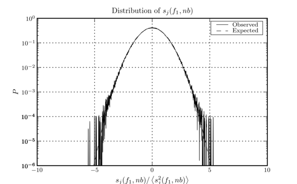
If the original time series is stationary Gaussian noise, this construction makes each frequency bin's real and imaginary parts Gaussian random variables with variances of 0.5. The definition of the power spectral density and of the Fourier transform shown above both match those of the LIGO Algorithm Library, as documented in LIGO-T010095-00-Z. Figure this figure shows the distribution of the real and imaginary components of \(\hat{s}_{k}\) obtained from a sample of \(h(t)\) taken from the LIGO L1 instrument during S4.
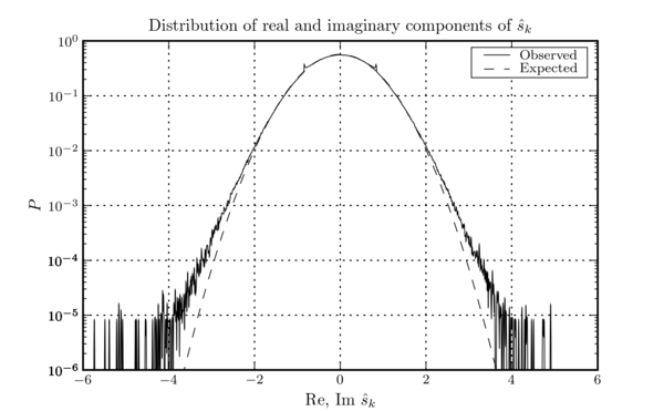
The distribution of the real and imaginary components of \(\hat{s}_{k}\) obtained from a sample of \(h(t)\) taken from the LIGO L1 instrument during S4. The aparent bias away from the expected normalization (actually non-Gaussianity) and the two horn features, are the result of correlations between the power spectrum and the data. Recall that the power spectrum is estimated from the same data it is used to whiten.
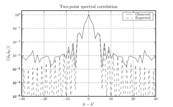
If the input time series is a stationary random process, then the components of its Fourier transform are uncorrelated, and we would find that \(\mean{\hat{s}_{k} \conj{\hat{s}}_{k'}} = \delta_{k k'}\). However, because we have windowed the time series (which is equivalent to convolving its Fourier transform with that of the window), the frequency components are now correlated. We can compute \(\mean{\hat{s}_{k} \conj{\hat{s}}_{k'}}\) by assuming the whitened time series consists of independently-distributed random variables, because then the Wiener-Khinchin theorem tells us that its two-point spectral correlation function is the Fourier transform of its variance which we'll assume is proportional to the square of the tapering window function. Therefore,
\begin{equation} \mean{\hat{s}_{k} \conj{\hat{s}}_{k'}} \propto \sum_{j = 0}^{N - 1} w_{j}^{2} \ee^{-2 \pi \aye j (k - k') / N}. \end{equation}
The proportionality constant is obtained from Eq. \eqref{eqn3}, which tells us that
\begin{equation} \label{eqn4} \mean{\hat{s}_{k} \conj{\hat{s}}_{k'}} = \frac{1}{\sigma_{w}^{2}} \sum_{j = 0}^{N - 1} w_{j}^{2} \ee^{-2 \pi \aye j (k - k') / N}. \end{equation}
A comparison of this prediction to the observed two-point spectral correlation in \(\hat{s}_{k}\) obtained from \(h(t)\) recorded at the LIGO L1 instrument during S4 is shown in this figure.
Using Eq. \eqref{eqn4} in place of the two-point spectral correlation function in Eq. \eqref{eqn9} allows us to compute the variance of the time series that results from inverse transforming the whitened frequency-domain data. This is
\begin{equation} \mean{s_{j}^{2}} = \frac{1}{\Delta t^{2} \sigma_{w}^{2}} w_{j}^{2}. \end{equation}
One finds the shape of the original window function preserved in the whitened time series.
The power spectral density is estimated using the median power at each frequency for a number of overlapping segments. The use of the median avoids bias in the spectrum caused by the presence of a gravitational wave or other large non-astrophysical transients present in any of the segments.
The choice of the channel filter is mostly irrelevant, except that it correspond in some meaningful way to a particular frequency band. We'll denote the channel filter spanning frequencyes \(f_{1} \leq f_{k} < f_{2}\) as \(\tilde{\Theta}_{k}(f_{1}, B)\), where the bandwidth of the filter is \(B = f_{2} - f_{1}\). If \(b\) is the bandwidth of the narrowest channel, excess power achieves a multi-resolution search by computing only the narrowest channels, and choosing
\begin{equation} \tilde{\Theta}_{k}(f_{1}, n b) = \sum_{i = 0}^{n - 1} \Theta_{k}(f_{1} + i b, b), \end{equation}
where \(B = n b\). That is, the filters for wide band channels are chosen to be the sums of adjacent filters from narrower bands. The specific choice made in excess power is to use Hann windows for the narrowest channels. The narrow channels are all the same width, and the Hann windows are adjusted to be centred on their channel and extend over a range of frequencies twice the width of the channel,
\begin{equation} \tilde{\Theta}_{k}(f_{1}, b) \propto \begin{cases} \sin^{2} \frac{\pi}{2 b} (f_{k} - f_{1} + \frac{b}{2}), & f_{1} - \frac{b}{2} \leq f_{k} < f_{1} + \frac{3 b}{2} \\ 0, & \text{othewise}. \end{cases} \end{equation}
In this way, when the filters for two adjacent channels are summed the result is a Tukey window — a window with a flat top in the middle and \(\sin^{2}\) tapers at each end.
All windows are real-valued, so that they are phase preserving. The narrowest channel filters, the filters of bandwidth \(b\), are normalized so that
\begin{equation} \label{eqn5} \sum_{k = 0}^{N - 1} \sum_{k' = 0}^{N - 1} -1^{(k - k')} \mean{\hat{s}_{k} \conj{\hat{s}}_{k'}} \conj{\tilde{\Theta}}_{k}(f_{1}, b) \tilde{\Theta}_{k'}(f_{1}, b) = \frac{b}{\Delta f}, \end{equation}
where the two-point spectral correlation is given in Eq. \eqref{eqn4}. The reason for this choice will become clear later. For convenience, let us introduce the notation
\begin{equation} \left\{ \tilde{X}, \tilde{Y} \right\} = \sum_{k = 0}^{N - 1} \sum_{k' = 0}^{N - 1} -1^{(k - k')} \mean{\hat{s}_{k} \conj{\hat{s}}_{k'}} \conj{\tilde{X}}_{k} \tilde{Y}_{k'}, \end{equation}
so
\begin{equation} \left\{ \tilde{\Theta}(f_{1}, b), \tilde{\Theta}(f_{1}, b) \right\} = \frac{b}{\Delta f}. \end{equation}
Notice that if the two-point spectral correlation is a Kroniker \(\delta\) (the input data is not windowed), and the channel filter is flat, \(\tilde{\Theta}_{k} = \tilde{\Theta}\), and spans the entire frequency band from DC to Nyquist, \(b / \Delta f = N\), then the normalization would lead to
\begin{equation} \tilde{\Theta} = 1. \end{equation}
In the LIGO Algorithm Library, the Fourier transforms of real-valued time series contain only postive frequency components (the negative frequency components being the complex conjugates of these), and so the channel filters are also stored as only positive frequency components. Since the two-point spectral correlation function is usually strongly-peaked around \(k - k' = 0\), and since the channel filters all go to zero far from the DC and Nyquist components, in practice it is safe to sum over only the positive frequency components, and require the sum to be
\begin{equation} 2 \sum_{k = 0}^{\lfloor N / 2 \rfloor + 1} \sum_{k' = 0}^{\lfloor N / 2 \rfloor + 1} -1^{(k - k')} \mean{\hat{s}_{k} \conj{\hat{s}}_{k'}} \conj{\tilde{\Theta}}_{k}(f_{1}, b) \tilde{\Theta}_{k'}(f_{1}, b) = \frac{b}{\Delta f}. \end{equation}
So the argument is that in practice this normalization is identical to Eq. \eqref{eqn5}, but it is easier to implement because these are the only components stored in memory.
For wide channels, channels formed by summing the filters from two or more narrow channels, the "magnitude" of the channel filter will not be \(n b / \Delta f\). For example,
\begin{equation} \tilde{\Theta}_{k}(f_{1}, 2 b) = \tilde{\Theta}_{k}(f_{1}, b) + \tilde{\Theta}_{k}(f_{1} + b, b), \end{equation}
and using the symmetry of \(\mean{\hat{s}_{k} \conj{\hat{s}}_{k'}}\) the magnitude of this channel filter is found to be
\begin{align} \left\{ \tilde{\Theta}(f_{1}, 2 b), \tilde{\Theta}(f_{1}, 2 b) \right\} & = \frac{2 b}{\Delta f} + 2 \left\{ \tilde{\Theta}(f_{1}, b), \tilde{\Theta}(f_{1} + b, b) \right\}. \end{align}
The channel construction described above, with Hann windows for the narrowest channels yielding Tukey windows for wider channels, allows us to make the approximation that only adjacent channel filters have sufficient overlap that their inner products are non-zero, and so the cross terms from adjacent channels are the only ones that need to be accounted for. Therefore, in general, a filter spanning \(n\) channels is
\begin{equation} \tilde{\Theta}_{k}(f_{1}, n b) = \sum_{i = 0}^{n - 1} \tilde{\Theta}_{k}(f_{1} + i b, b), \end{equation}
and its magnitude is
\begin{equation} \left\{ \tilde{\Theta}(f_{1}, n b), \tilde{\Theta}(f_{1}, n b) \right\} = \frac{n b}{\Delta f} + 2 \sum_{i = 0}^{n - 2} \left\{ \tilde{\Theta}(f_{1} + i b, b), \tilde{\Theta}(f_{1} + (i + 1) b, b) \right\}. \end{equation}
Let us denote this magnitude as \(\mu^{2}(f_{1}, n b)\),
\begin{equation} \label{eqn2} \mu^{2}(f_{1}, n b) = \frac{n b}{\Delta f} + 2 \sum_{i = 0}^{n - 2} \sum_{k = 0}^{N - 1} \sum_{k' = 0}^{N - 1} -1^{(k - k')} \mean{\hat{s}_{k} \conj{\hat{s}}_{k'}} \tilde{\Theta}_{k}(f_{1} + i b, b) \conj{\tilde{\Theta}}_{k'}(f_{1} + (i + 1) b, b). \end{equation}
When \(n = 1\), \(\mu^{2} = b / \Delta f\).
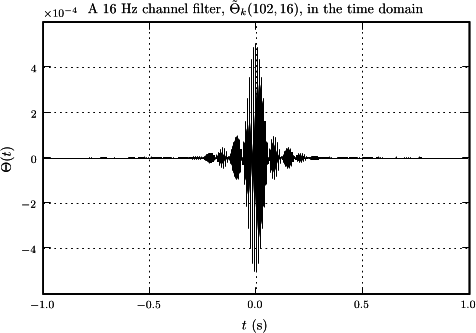
this figure illustrates the construction of a 16 Hz channel filter from four 4 Hz channel filters when \(\mean{\hat{s}_{k} \conj{\hat{s}}_{k'}} = \delta_{k k'}\).
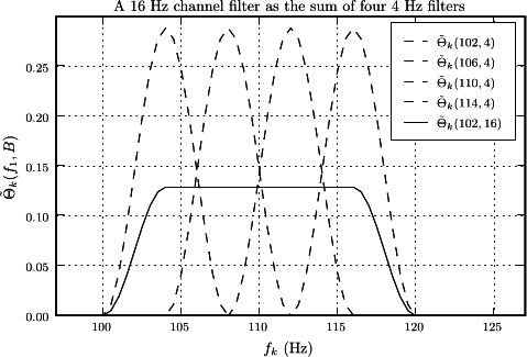
The 16 Hz channel filter has had its normalization adjusted by the factor in Eq. \eqref{eqn2} to illustrate the relative amplitudes of the channel filters when all are normalized to have magnitudes of 1. This figure also shows how the approximation that only adjacent channels have non-zero overlap becomes exact in the limit of a two-point spectral correlation function that is a Kroniker \(\delta\) (the "tapering" window is flat, \(w_{j} = 1\)), because the third channel filter can only overlap the first when there is mixing between \(k\). The time-domain versions of two sample channel filters are shown in this figure.
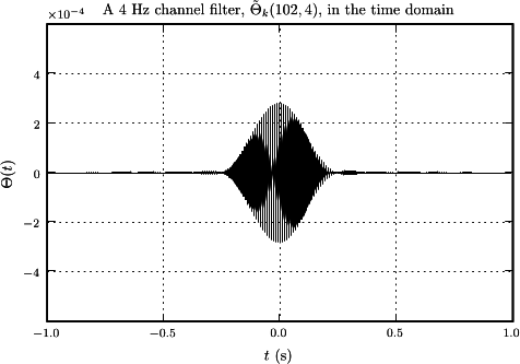
The time series for a channel is extracted by multiplying the whitened frequency-domain input data by the channel filter, and transforming the result back to the time domain. The time series for the channel of bandwidth \(b\) starting at frequency \(f_{1}\) is
\begin{equation} \label{eqn1} z_{j}(f_{1}, b) = \frac{1}{N \Delta t} \sum_{k = 0}^{N - 1} \hat{s}_{k} \conj{\tilde{\Theta}}_{k}(f_{1}, b) \ee^{2 \pi \aye j k / N}, \end{equation}
and the mean square is
\begin{equation} \mean{z_{j}^{2}(f_{1}, b)} = \frac{1}{N^{2} \Delta t^{2}} \sum_{k = 0}^{N - 1} \sum_{k' = 0}^{N - 1} \mean{\hat{s}_{k} \conj{\hat{s}}_{k'}} \conj{\tilde{\Theta}}_{k}(f_{1}, b) \tilde{\Theta}_{k'}(f_{1}, b) \ee^{2 \pi \aye j (k - k') / N}. \end{equation}
The mean square is sample-dependent (depends on \(j\)) because the original time series had the window \(w_{j}\) applied to it. We will now require that the window be of a kind with a flat portion in the middle, so that
\begin{equation} w_{j} = \begin{cases} 1 & \text{if $0 \leq j_{1} \leq j < j_{2} \leq N$}, \\ \leq 1 & \text{otherwise}. \end{cases} \end{equation}
For example, a Tukey window is suitable. In that case, the mean square of \(z_{j}(f_{1}, b)\) should be independent of \(j\) when \(j_{1} \leq j < j_{2}\). If we further require the flat portion of the window to be in the middle, in other words require \(j_{1}\) and \(j_{2}\) to be such that \(j_{1} \leq N / 2 < j_{2}\), then we can pick \(j = N / 2\) as representative of the mean square of \(z_{j}(f_{1}, b)\) in the flat portion of the window. Therefore,
\begin{equation} \mean{z_{j}^{2}(f_{1}, b)} = \frac{1}{N^{2} \Delta t^{2}} \sum_{k = 0}^{N - 1} \sum_{k' = 0}^{N - 1} -1^{(k - k')} \mean{\hat{s}_{k} \conj{\hat{s}}_{k'}} \conj{\tilde{\Theta}}_{k}(f_{1}, b) \tilde{\Theta}_{k'}(f_{1}, b). \end{equation}
From the normalization of the channel filters (the motivation for the formulation of which is now seen), the sum is \(b / \Delta f\), and therefore
\begin{equation} \mean{z_{j}^{2}(f_{1}, b)} = \frac{1}{N^{2} \Delta t^{2}} \frac{b}{\Delta f}, \end{equation}
for \(j_{1} \leq j < j_{2}\).
The LIGO Algorithm Library's XLALREAL4ReverseFFT() function computes the inverse transform omitting the factor of \(\Delta f = 1 / (N
\Delta t)\) that appears in Eq. \eqref{eqn1}. The time series returned by this function is
\begin{equation} Z_{j}(f_{1}, b) = N \Delta t z_{j}(f_{1}, b), \end{equation}
and the mean squares of the samples in the time series are
\begin{equation} \mean{Z_{j}^{2}(f_{1}, b)} = \frac{b}{\Delta f}, \end{equation}
for \(j_{1} \leq j < j_{2}\). For a channel spanning \(n\) narrow channels,
\begin{align} Z_{j}(f_{1}, n b) & = \sum_{k = 0}^{N - 1} \hat{s}_{k} \conj{\tilde{\Theta}}_{k}(f_{1}, n b) \ee^{2 \pi \aye j k / N} \\ & = \sum_{k = 0}^{N - 1} \hat{s}_{k} \left( \sum_{i = 0}^{n - 1} \conj{\tilde{\Theta}}_{k}(f_{1} + i b, b) \right) \ee^{2 \pi \aye j k / N} \\ & = \sum_{i = 0}^{n - 1} Z_{j}(f_{1} + i b, b), \end{align}
and so the samples in the time series for a wide channel are obtained by summing the samples from the appropriate narrow channel time series. The mean squares of the samples of a wide channel's time series are given by the quantity in Eq. \eqref{eqn2},
\begin{equation} \mean{Z_{j}^{2}(f_{1}, n b)} = \mu^{2}(f_{1}, n b). \end{equation}
this figure shows the distribution of \(Z_{j}(f_{1}, B)\) observed in the same data used to measure the \(\hat{s}_{k}\) distribution in this figure.
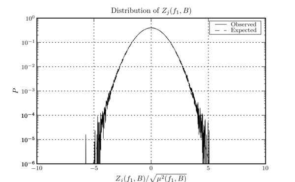
This distribution appears more Gaussian than does the distribution of the real and imaginary components of the whitened frequency series, and generally exhibits better agreement with its expected behaviour. Presumably this is a result of the central limit theorem: the real and imaginary components of the whitened frequency series may not be Gaussian, but they do have unit variance, and since the time-domain samples of \(Z_{j}\) are computed from many thousands of frequency bins, they end up being unit variance Gaussian random variables.
Having projected the whitened input time series onto a comb of frequency channels, including channels with a variety of widths, we now procede to project it onto a collection of time-frequency tiles. For this, we need to know that the number of degrees of freedom in a tile of bandwidth \(B\) and duration \(T\) is
\begin{equation} d = 2 B T. \end{equation}
This can be understood as follows. A real-valued signal with a bandwidth of \(B\) can be represented without loss of information as a discrete real-valued time series with a sample rate equal to the Nyquist frequency \(2 B\) (the time series may be a heterodyned version of the signal). Therefore, \(2 B T\) real-valued samples are sufficient to encode all the information contained in a signal of bandwidth \(B\) and duration \(T\). We will require the number of degrees of freedom to be an even integer not less than 2.
To construct the time-frequency tile spanning the frequencies \(f_{1} \leq f < f_{1} + B\), and the times \(t_{1} \leq t < t_{1} + T\), we will use the samples from the channel time series \(Z_{j}(f_{1}, B)\). The channel time series' sample period is \(\Delta t\), the same sample period as the original input time series, but because the channel time series corresponds to a more narrow frequency band than does the original input time series (except in the special case of a channel spanning the entire input band), there are more samples per unit time in the channel time series than there are degrees of freedom per unit time — the channel time series is over sampled. To obtain a time series with the correct sample rate, a sample rate matching the actual number of degrees of freedom per second, we need to down-sample the channel time series.
Let \(j_{1} = t_{1} / \Delta t\) be the time series sample index corresponding to the start time of the tile. The tile's duration spans a total of \(T / \Delta t\) samples in the channel time series, but the tile has \(d\) degrees of freedom so we need to down-sample the channel time series so that from the \(T / \Delta t\) samples starting at \(j_{1}\) we are left with \(d\) linearly independent numbers. A simple down sampling procedure is to select \(d\) evenly-spaced samples from the \(T / \Delta t\) samples starting at \(j_{1}\). Let these be the \(d\) samples at the indices
\begin{equation} \label{eqn8} j = j_{1} + (i + \frac{1}{2}) \Delta j, \end{equation}
where \(i = 0, \ldots, d - 1\), and \(\Delta j = T / (d \Delta t)\). These samples are linearly independent in the sense that it is not possible to compute any one of them from the \(d - 1\) other samples, but they are correlated because of the impulse response of the channel filter in the time domain. See, for example, this figure. In what follows we will need the \(d\) samples forming the time-frequency tile to be independent Gaussian random variables when the input time series is stationary Gaussian noise.
Let us say that our \(d\) samples are the result of convolving the channel impulse response with the "real" samples, and assume that if we deconvolve the channel's impulse response from our samples we will be left with \(d\) independent random variables. The impulse response is proportional to the inverse Fourier transform of the channel filter,
\begin{equation} \Theta_{j}(f_{1}, B) = \frac{1}{N \Delta t} \sum_{k = 0}^{N - 1} \tilde{\Theta}_{k}(f_{1}, B) \ee^{2 \pi \aye j k / N}. \end{equation}
Labeling the "real" samples as \(Z_{j}'(f_{1}, B)\), our assumption is that our samples are derived from them by
\begin{equation} \begin{bmatrix} \vdots \\ Z_{j}(f_{1}, B) \\ \vdots \end{bmatrix} \propto \begin{bmatrix} & \vdots & \\ \cdots & \Theta_{j - j'}(f_{1}, B) & \cdots \\ & \vdots & \end{bmatrix} \begin{bmatrix} \vdots \\ Z_{j'}'(f_{1}, B) \\ \vdots \end{bmatrix}, \end{equation}
where the \(j\) and \(j'\) indices are taken from Eq. \eqref{eqn8}. Let's write this matrix equation as
\begin{equation} \vec{Z}(f_{1}, B) \propto \bar{\Theta}(f_{1}, B) \cdot \vec{Z}'(f_{1}, B). \end{equation}
Inverting the equation gives the "real" samples in terms of our measured samples,
\begin{equation} \vec{Z}'(f_{1}, B) \propto \bar{\Theta}^{-1}(f_{1}, B) \cdot \vec{Z}(f_{1}, B). \end{equation}
The proportionality constant is obtained by demanding that \(\mean{Z_{j'}'^{2}(f_{1}, B)} = 1\).
We define the whitened energy contained in the tile spanning the frequencies \(f_{1} \leq f < f_{1} + B\) and the times \(t_{1} \leq t < t_{1} + T\) as the sum of the squares of the down-sampled channel time series
\begin{align} E & = \frac{1}{\mu^{2}(f_{1}, B)} \vec{Z}(f_{1}, B) \cdot \vec{Z}(f_{1}, B) \\ \label{eqn6} & = \frac{1}{\mu^{2}(f_{1}, B)} \sum_{i = 0}^{d - 1} Z_{j_{1} + (i + \frac{1}{2}) \Delta j}^{2}(f_{1}, B), \end{align}
where \(j_{1} = t_{1} / \Delta t\) is the time series index corresponding to the start of the tile, and \(\Delta j = T / (d \Delta t)\) is the number of time series samples separating pixels in the time-frequency tile.
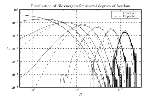
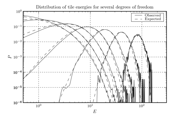
When the input time series is stationary Gaussian noise, \(E\) is the sum of the squares of \(d\) Gaussian random variables each of whose mean is 0 and whose mean square is 1 (the factor of \(\mu^{2}\) normalizes them). Therefore, \(E\) should be a \(\chi^{2}\)-distributed random variable of \(d\) degrees of freedom. Having measured an \(E\) for a tile, we can calculate the probability that a tile would be found with at least that \(E\) in stationary Gaussian noise, and threshold on this probability. We discard all tiles except those for which this probability is close to 0. The tiling results in a large number of tiles being tested in every second of data, and so a practical threshold is \(P(\geq E) \sim 10^{-7}\), yielding an event rate of \(\order(\text{few})\) Hz. Figure this figure shows a histogram of whitened tile energies observed in the same strain data used to generate this figure and this figure.
When a tile is identified as being unusual, the event is recorded in the output file, and several properties of the event are measured and recorded. One property is the "confidence", defined as
\begin{equation} \text{confidence} = -\ln P(\geq E), \end{equation}
the negative of the natural logarithm of the probability of observing a tile with a whitened energy of \(E\) or greater in stationary Gaussian noise. This probability is typically close to 0, so the natural logarithm is a large negative number, and the confidence a large positive number. Larger "confidence" means a tile less like one would find in stationary Gaussian noise. A second quantity recorded for each event is the signal-to-noise ratio (SNR). The "excess power" (really excess energy), of an event is
\begin{equation} \text{excess power} = E - d. \end{equation}
The expectation value of the whitened energy is \(\mean{E} = d\), so \(E - d\) is the amount of whitened energy in the time-frequency tile beyond what was expected — the "signal". Since the expected whitened energy is \(d\), the SNR is
\begin{equation} \rho = \frac{E - d}{d}. \end{equation}
The final quantity recorded for each event is the root-sum-squared strain, or \(h_{\text{rss}}\). We want the \(h_{\text{rss}}\) associated with a particular time-frequency tile, and to do this we would like to have the strain time series for the channel from which the time-frequency tile has been constructed, \(h_{j}(f_{1}, B)\). Unfortunately, we don't have this information because we don't know what of the data is noise and what is gravitational wave strain. However, if we assume that the strain time series and the noise time series are independent of one another, then the mean square of data time series is the sum of the mean squares of the strain and gravitational wave time series,
\begin{equation} \mean{s_{j}^{2}(f_{1}, B)} = \mean{h_{j}^{2}(f_{1}, B)} + \mean{n_{j}^{2}(f_{1}, B)}. \end{equation}
This is true on average, but we can use it to estimate the sum-of-squares of \(h\) by summing the squares of \(s\) and subtracing the estimate of the sum-of-squares of \(n\) derived from the measured power spectral density. Essentially, we measure the "energy" in a time-frequency tile, and subtract the mean noise energy to leave us with the gravitational wave strain energy. Therefore,
\begin{align} \sum_{d} h_{j}^{2}(f_{1}, B) & = \left( \sum_{d} s_{j}^{2}(f_{1}, B) \right) - d \mean{n_{j}^{2}(f_{1}, B)} \\ & = \left( \sum_{d} s_{j}^{2}(f_{1}, B) \right) - d \mean{s_{j}^{2}(f_{1}, B)}. \end{align}
In this last line the notation has gotten a little confusing. There is the actual sum of squares of the data, and there is the expected sum of squares. We are using the (measured) mean square of the data in place of the mean square of the noise on the assumption that it is noise that dominates this quantity. Also, \(\sum_{d}\) indicates the sum of \(d\) time samples whose indices are the same as was used in Eq. \eqref{eqn6}.
The unwhitened time series corresponding to a single frequency channel is the inverse Fourier transform of the unwhitened frequency series input data multiplied by the corresponding channel filter,
\begin{align} s_{j}(f_{1}, b) & = \frac{1}{N \Delta t} \sum_{k = 0}^{N - 1} \tilde{s}_{k} \conj{\tilde{\Theta}}_{k}(f_{1}, b) \ee^{2 \pi \aye j k / N} \\ & = \frac{1}{N \Delta t \sqrt{2 \Delta f}} \sum_{k = 0}^{N - 1} \sqrt{P_{k}} \hat{s}_{k} \conj{\tilde{\Theta}}_{k}(f_{1}, b) \ee^{2 \pi \aye j k / N} \\ \label{eqn7} & = \frac{1}{\sqrt{2 N \Delta t}} \sum_{k = 0}^{N - 1} \sqrt{P_{k}} \hat{s}_{k} \conj{\tilde{\Theta}}_{k}(f_{1}, b) \ee^{2 \pi \aye j k / N}. \end{align}
For a wide channel, \(\tilde{\Theta}_{k}(f_{1}, n b)\), we find just as for \(Z_{j}(f_{1}, n b)\), that
\begin{equation} s_{j}(f_{1}, n b) = \sum_{i = 0}^{n - 1} s_{j}(f_{1} + i b, b). \end{equation}
The mean square of the unwhitened time series for a single channel is
\begin{equation} \mean{s_{j}^{2}(f_{1}, b)} = \frac{1}{2 N \Delta t} \sum_{k = 0}^{N - 1} \sum_{k' = 0}^{N - 1} \sqrt{P_{k} P_{k'}} \mean{\hat{s}_{k} \conj{\hat{s}}_{k'}} \conj{\tilde{\Theta}}_{k}(f_{1}, b) \tilde{\Theta}_{k'}(f_{1}, b) \ee^{2 \pi \aye j (k - k') / N}. \end{equation}
Making the same assumption as before, that the time series' mean square is independent of the sample index \(j\) in the flat part of the input tapering window, we can set \(j = N / 2\) inside the sum to leave us with
\begin{equation} \mean{s_{j}^{2}(f_{1}, b)} = \frac{1}{2 N \Delta t} \sum_{k = 0}^{N - 1} \sum_{k' = 0}^{N - 1} -1^{(k - k')} \sqrt{P_{k} P_{k'}} \mean{\hat{s}_{k} \conj{\hat{s}}_{k'}} \conj{\tilde{\Theta}}_{k}(f_{1}, b) \tilde{\Theta}_{k'}(f_{1}, b). \end{equation}
The double sum is a spectral density weighted version of the inner product defined earlier for channel filters. Introducing the notation
\begin{equation} \left\{ X, Y; P \right\} = \sum_{k = 0}^{N - 1} \sum_{k' = 0}^{N - 1} -1^{(k - k')} \sqrt{P_{k} P_{k'}} \mean{\hat{s}_{k} \conj{\hat{s}}_{k'}} \conj{X}_{k} Y_{k}, \end{equation}
we can write the mean square as
\begin{equation} \mean{s_{j}^{2}(f_{1}, b)} = \frac{1}{2 N \Delta t} \left\{ \tilde{\Theta}(f_{1}, b), \tilde{\Theta}(f_{1}, b); P \right\}. \end{equation}
If we again make the assumption that only adjacent channels have any significant non-zero overlap, then the mean square of the samples in an unwhitened wide channel is
\begin{equation} \mean{s_{j}^{2}(f_{1}, n b)} = \sum_{i = 0}^{n - 1} \mean{s_{j}^{2}(f_{1} + i b, b)} + \frac{1}{N \Delta t} \sum_{i = 0}^{n - 2} \left\{ \tilde{\Theta}(f_{1} + i b, b), \tilde{\Theta}(f_{1} + (i + 1) b, b) ; P \right\}. \end{equation}
We need the \(s_{j}(f_{1}, n b)\) time series in order to compute the unwhitened sum-of-squares for a particular tile, but constructing this time series explicitly with the likes of Eq. \eqref{eqn7} incurs a factor of 2 cost in both time and memory. An approximation that works well in practice is to assume that single channels of bandwidth \(b\) are sufficiently narrow that the power spectral density is approximately constant in each one. This allows \(P_{k}\) in Eq. \eqref{eqn7} to be replaced with some sort of average and factored out of the sum to leave
\begin{equation} s_{j}(f_{1}, b) \propto Z_{j}(f_{1}, b). \end{equation}
The constant of proportionality is obtained from the known mean squares of \(s_{j}(f_{1}, b)\) and \(Z_{j}(f_{1}, b)\), both of which are computed (almost) without approximation. Therefore,
\begin{equation} s_{j}(f_{1}, b) \approx \sqrt{\frac{\Delta f}{b}} \sqrt{\mean{s_{j}^{2}(f_{1}, b)}} Z_{j}(f_{1}, b). \end{equation}
We compute \(s_{j}(f_{1}, n b)\) for a wide channel by summing samples across narrow channels,
\begin{equation} s_{j}(f_{1}, n b) = \sum_{i = 0}^{n -1} s_{j}(f_{1} + i b, b) \propto \sqrt{\frac{\Delta f}{b}} \sum_{i = 0}^{n -1} \sqrt{\mean{s_{j}^{2}(f_{1} + i b, b)}} Z_{j}(f_{1} + i b, b), \end{equation}
and again we solve for the proportionality constant from the ratio of the mean squares of the left- and right-hand sides. The mean square of the left-hand side is given above, and that of the right-hand side is
\begin{multline} \mean{\left( \sqrt{\frac{\Delta f}{b}} \sum_{i = 0}^{n -1} \sqrt{\mean{s_{j}^{2}(f_{1} + i b, b)}} Z_{j}(f_{1} + i b, b) \right)^{2}} = \sum_{i = 0}^{n -1} \mean{s_{j}^{2}(f_{1} + i b, b)} \\+ \frac{2 \Delta f}{b} \sum_{i = 0}^{n - 2} \sqrt{\mean{s_{j}^{2}(f_{1} + i b, b)} \mean{s_{j}^{2}(f_{1} + (i + 1) b, b)}} \left\{ \tilde{\Theta}(f_{1} + i b, b), \tilde{\Theta}(f_{1} + (i + 1) b, b) \right\}. \end{multline}
Denoting the ratio as
\begin{equation} \Upsilon^{2}(f_{1}, n b) = \mean{s_{j}^{2}(f_{1}, n b)} \mean{\left( \sum_{i = 0}^{n -1} \sqrt{\mean{s_{j}^{2}(f_{1} + i b, b)}} Z_{j}(f_{1} + i b, b) \right)^{2}}^{-1}, \end{equation}
the approximate unwhitened time series is
\begin{equation} s_{j}(f_{1}, n b) \approx \sqrt{\Upsilon^{2}(f_{1}, n b)} \sqrt{\frac{\Delta f}{b}} \sum_{i = 0}^{n -1} \sqrt{\mean{s_{j}^{2}(f_{1}, b)}} Z_{j}(f_{1}, b). \end{equation}
this figure shows a comparison of the distribution observed in the samples of the approximate unwhitened time series \(s_{j}(f_{1}, n b)\) values, for all bandwidths, as derived from the same sample of \(h(t)\) recorded at the LIGO Livingston L1 instrument during S4 that has been used for the other plots.
Finally,
\begin{equation} \sum_{j} h_{j}^{2}(f_{1}, n b) \Delta t = \sum_{j} s_{j}^{2}(f_{1}, n b) \Delta t - d \mean{s_{j}^{2}(f_{1}, n b)} \Delta t, \end{equation}
so,
\begin{equation} h_{\text{rss}} = \sqrt{\sum_{j} s_{j}^{2}(f_{1}, n b) \Delta t - d \mean{s_{j}^{2}(f_{1}, n b)} \Delta t}. \end{equation}
A example of the results can be see in this figure.
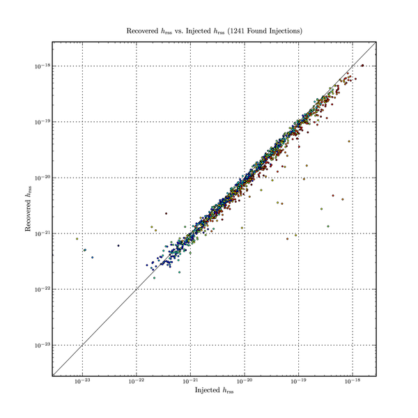
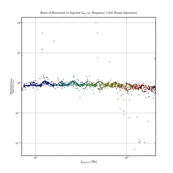
It must be remarked that this procedure can occasionally yield an estimated \(h_{\text{rss}}\) that is not real-valued. This happens when the observed unwhitened energy, \(\sum_{j} s_{j}^{2} \Delta t\), proves to be less than the expected unwhitened energy, \(d \mean{s_{j}^{2}} \Delta t\). The whitened energy is always greater than the expected amount by construction because we threshold on it, discarding any tiles below some cut-off. Another way of expressing this is to say that the whitened SNR is always greater than 1, but the unwhitened SNR need not be. This should not be unexpected because the arithmetic by which the frequency-domain data is turned into a whitened and unwhitened sum-squares weights different frequency bins differently. In particular, non-real \(h_{\text{rss}}\) values are seen more frequency in the vicinity of strong line features such as the violin modes, where the difference between the whitened and unwhitened spectra are the greatest. The search code discards any tiles whose estimated \(h_{\text{rss}}\) is not real-valued.
this section began with the comment that the choice of channel filter is mostly irrelevant, so long as there is some sense in which it corresponds to a particular frequency band. In the derivations that followed, the approximation was made that only adjacent channel filters have any appreciable overlap. A particular choice of channel filter was described, but other choices are possible. One improvement that can be made is to identify lines in the spectral density, and add notches to the channel filters to remove them. Often these spectral line features are the result of noise processes in the instrument or its environment. For example, suspension wire resonances, harmonics of the 60 Hz power line frequency, and optic resonances are all prominently visible in the spectrum of LIGO interfermeter. The effect of adding notches at these frequencies is to cause the search to measure the energy in the time-frequency tiles preferentially from those frequency bands less contaminated by these noise sources.
A simple way of deweighting contaminated frequency bands is to divide the channel filters by some power of the power spectral density,
\begin{equation} \tilde{\Theta}_{k}'(f_{1}, B) \propto P_{k}^{-a} \tilde{\Theta}_{k}(f_{1}, B). \end{equation}
The modified channel filters are normalized as before. When \(a = \frac{1}{2}\), that is the nominal channel filters are divided by the square root of the power spectral density, the procedure is called "over whitening". There are, aparently, theoretical reasons to make this choice. Over-whitening is found to significantly improve the ability of the excess power search to reject noise, and so the actual channel filters used by the search are not only the Hann windows described above but also contain one inverse power of the square root of the power spectral density.
The excess power analysis code does not process the input data as a continuous time series; rather the time series is split into a sequence of discrete "analysis windows", which are each analyzed individually. To account for the possibility of a burst event stradling the boundary between two analysis windows, successive windows are staggered in such a way that they overlap one another in time. In this way, a burst event occuring on the boundary of one window will (typically) be centred in the next.
Because edge effects at various stages of the analysis can corrupt the beginning and end of the analysis window, the actual quantity of data extracted from the input time series to form a window is twice the amount that is analyzed. Only results from the central half of the window are retained, with the first and last quarters of each window being discarded. The arrangement is shown in the following diagram.

Here we see a discrete time series (represented by the bottom-most horizontal line) that contains 57344 samples. It has been divided into a sequence of four analysis windows, each containing 32768 samples. A fifth, greyed-out, analysis window is shown to indicate where the next window in the sequence would start. In the analysis of each window, the first and last 8192 samples (first and last quarter) are discarded as indicated by the crossed-out sections in each window. In this particular example, each window is shifted 8192 samples (also equal to one quarter of the window length) from the start of the previous window. This choice of window length and window shift causes the sections of each window that are actually searched for events (the sections that are not crossed out) to overlap their neighbours by half of their own width. This is the typical mode of operation for the search code. Notice that the first and last quarter window length of the complete time series (the cross-out sections in the bottom line) are not analyzed, as they are discarded from the only analysis windows in which they appear.
The excess power code whitens the input time series using an estimate of the instrument's noise power spectral density (PSD). The estimated noise PSD is computed by averaging the PSDs from a number of successive analysis windows. The noise PSD is not estimated by averaging over the entire time series in order to allow the code to track the (possibly) changing character of the instrument's noise. For convenience, the user is permitted to enter the number of samples that should be used to estimate the PSD. The number of samples entered should correspond to the time for which the instrument's noise can be approximated as stationary for the purpose of the excess power analysis. Since, however, the actual estimation procedure involves averaging over an integer number of analysis windows, it is necessary for the number of samples selected to correspond to the boundary of an analysis window. For convenience, lalapps_power will automatically round the value entered down to the nearest analysis window boundary.
The LAL function EPSearch() performs the parts of the analysis described above. It is given a time series that it divides into analysis windows, which it uses to estimate the noise PSD. Using the estimated noise PSD, it whitens each analysis window and then searches them for burst events. Only the analysis windows within the data used to estimate the noise PSD are whitened using that estimate. Once those windows have been searched for burst events, EPSearch() returns to the calling procedure which then extracts a new time series from the input data and the process repeats. The parameter provided via the command line option –psd-average-points sets the length of the time series that is passed to EPSearch().
As successive time series are passed to EPSearch(), in order for the first analysis window to correctly overlap the last window from the previous time series — i.e. to ensure the same overlap between analysis windows in neighbouring time series as exists between neighbouring windows within a series — it is necessary for the latter time series to begin \((\mbox{<i>window length</i>} - \mbox{<i>window shift</i>})\) samples before the end of the former series. The arrangement is shown in the following figure.

Here we see two of the time series from the first diagram above, each of which is to be passed to EPSearch() for analysis. To see why the overlap between these two time series must be chosen as it is, refer to the first diagram above to see where the greyed-out fifth analysis window was to be placed. That is where the first analysis window in the second time series here will be placed.
Prior to looping over the data one noise PSD estimation length at a time, the data is passed through a conditioning filter. To account for edge effects in the filter, an amount of data set by the command line option –filter-corruption is dropped from the analysis at both the begining and end of the time series. The arrangement is shown in the following diagram.

The bottom-most line in this diagram represents the time series as read into memory from disk. In this example we have read 106496 samples into memory, and after passing it through the conditioning filter 8192 samples are dropped from the beginning and end of the series. The remaining data is then passed to EPSearch() 57344 samples at a time — just as was done in the earlier examples — with appropriate overlaps. In this example, it happens that an integer number of overlaping noise PSD intervals fits into the data that survives the conditioning. In general this will not be the case. If the last noise PSD interval would extend beyond the end of the time series, it is moved to an earlier time so that its end is aligned with the end of the available data.
If more data needs to be analyzed than will fit in RAM at one time, we must read it into memory and analyze it in pieces. In doing this, we again want the analysis windows in neighbouring read cycles to overlap one another in the same manner that neighbouring analysis windows within a single noise PSD interval overlap one another. This will be assured if, in the diagram above, the start of the next data to be read from disk is arranged so that the first noise PSD interval to be analyzed within it starts at the correct location relative to the last PSD interval analyzed from the previous read cycle. Consideration of the diagram above reveals that in order to meet this condition, the next data to be read into memory should start \((2 \times \mbox{<i>filter corruption</i>} + \mbox{<i>window length</i>} - \mbox{<i>window shift</i>})\) samples prior to the end of the previous data to have been read.
lalapps_binj — produces burst injection data files.
lalapps_binj –gps-start-time seconds –gps-end-time seconds [–help] [–max-amplitude value] [–min-amplitude value] [–max-bandwidth Hertz] [–min-bandwidth Hertz] [–max-duration seconds] [–min-duration seconds] [–max-e-over-r2 \(\Msol/\text{\parsec}^{2}\)] [–min-e-over-r2 \(\Msol/\text{\parsec}^{2}\)] [–max-frequency Hertz] [–min-frequency Hertz] [–output filename] [–population name] [–q value] [–ra-dec radians,radians] [–seed value] [–time-step value] –time-slide-file filename [–user-tag string]
lalapps_binj produces a LIGO Light-Weight XML file containing a sim_burst table describing a sequence of burst software injections. This file can be read by lalapps_power and lalapps_StringSearch, which will perform the software injections described therein while analyzing data.
lalapps_binj produces one of three injection populations: an injection population simulating cosmological string cusp burst events, an injection population consisting of sine-Gaussians uniformly distributed over the sky, and an injection population of band- and time-limited white-noise burst waveforms originating from a specific location on the sky. These populations are selected with the –population option. Each population required additional parameters to characterize it, and other command line options are associated with these.
The output is written to a file name in the standard burst pipeline format:
where USERTAG is the user tag specfied on the command line, and GPSSTART and DURATION describes the GPS time interval that the file covers. If a –user-tag is not specified on the command line, the _USERTAG part of the filename will be omitted.
sim_burst injections can be performed into non-zero-lag data. The vector of time offsets to be applied to the instruments is stored in a time_slide table, and each sim_burst injection carries a time_slide_id to indicate the appropriate vector. Note that the actual time of the injection in each instrument is obtained by subtracting the offsets from the times recorded in the sim_burst table. This convention is used for consistency with the interpretation of use of vectors for burst<-->burst coincidences: if the offsets are subtracted from the injection times to obtain the actual times in the instruments, then when the same offset vector is added to the times of the triggers that result from the injection (as will be done by the coincidence code) they will re-align and form a coincidence.
–gps-end-time secondsSet the end time of the injection population in GPS seconds. The injection list in the output file will contain injections that span only the times between –gps-start-time and –gps-end-time.
–gps-start-time secondsSet the start time of the injection population in GPS seconds. The injection list in the output file will contain injections that span only the times between –gps-start-time and –gps-end-time.
–helpPrint a usage message.
–max-amplitude valueSet the upper bound of the range of injection amplitudes. This only affects string cusp injections.
–min-amplitude valueSet the lower bound of the range of injection amplitudes. This only affects string cusp injections.
–max-bandwidth HertzSet the upper bound of the range of injection bandwidths. This only affects band- and time-limited white-noies burst injections.
–min-bandwidth HertzSet the lower bound of the range of injection bandwidths. This only affects time- and band-limited white-noise burst injections.
–max-duration secondsSet the upper bound of the range of injection durations. This only affects time- and band-limited white-noise burst injections.
–min-duration secondsSet the lower bound of the range of injection durations. This only affects time- and band-limited white-noise burst injections.
–max-e-over-r2 \(\Msol / \text{\parsec}^{2}\)Set the upper bound of the range of injection energies. This only affects time- and band-limited white-noise burst injections. The energy of the injection is the equivalent isotropic radiated energy at the source, and since the strain at Earth depends not only on total energy radiated but also the distance to the source the value given here on the command line is the energy divided by the distance squared. Furthermore, since the energy radiated is proportional to the square of the derivative of the strain, higher frequency injections are harder to detect (the higher frequency means that the same energy is achieved with a smaller total strain, additionally interferometer detectors experience greater shot noise at high frequency). Therefore, so that the injections are appoximately equally detectable across the band, the energy range set on the command line is scaled by \((f / 100~\text{Hz})^{3}\) (the range given on the command line is exactly the range of energies at 100 Hz; the exponent is found impirically).
–min-e-over-r2 \(\Msol / \text{\parsec}^{2}\)Set the lower bound of the range of injection energies. This only affects time- and band-limited white-noise burst injections. See –max-e-over-r2 for more information.
–max-hrss valueSet the upper bound of the range of injection \(h_{\text{rss}}\) values. This only affects sine-Gaussian injections. Infact, this argument sets the product of the injection's \(h_{\text{rss}}\) and its duration — shorter injections will be assigned higher \(h_{\text{rss}}\) values. This improves the match of the injection amplitudes to the pipeline's sensitivity curve. The "duration" of a sine-Gaussian is interpreted to be \(Q / (\sqrt{2} \pi f)\).
–min-hrss valueSet the lower bound of the range of injection \(h_{\text{rss}}\) values. This only affects sine-Gaussian injections. See –max-hrss for more information.
–output filenameSet the name of the output file. The default complies with the file naming convention described in LIGO-T010150-00-E. Try for yourself to see what it does. If the filename ends in .gz it will be gzip compressed.
–population nameSelect the injection population. The allowed names are targeted, string_cusp, all_sky_sinegaussian.
–q valueSet the \(Q\) of the injections. This only affects sine-Gaussian injections.
–ra-dec radians,radiansSet the right-ascension and declination of the sky location from which injections should originate when generating a targeted population. Co-ordinates are in radians.
–seed valueSet the seed for the random number generator. This allows an injection population to be reconstructed identically, or to ensure that two different files do not contain the same injections.
–time-step valueSet the time interval between injections in seconds.
–time-slide-file filenameSet the name of the LIGO Light-Weight XML file from which to load the time slide table. The document must contain exactly 1 time slide vector, and only the contents of the process, process_params, search_summary (optional), sim_burst (optional), and time_slide tables will be copied into lalapps_binj's output.
–user-tag stringThe program ligolw_bucluster ("burst cluster") applies a clustering alogrithm to the burst events stored in the sngl_burst tables of one or more LIGO light weight XML files. At this time only one clustering algorithm is implemented, the clustering algorithm used by the excess power burst search pipeline. For more information on running this program, consult its usage message.
The excess power search is a multi-resolution analysis of the time-frequency structure of the input time series. A burst trigger is identified if the probability of obtaining the observed energy in the same time-frequency tile in Gaussian noise is smaller than some threshold. A large burst in the data stream will result in many nearby time-frequency tiles being identified as triggers, all with different sizes and aspect ratios, many overlapping one another. The program ligolw_bucluster replaces these moguls of triggers with single triggers intended to summarize the event. The following clustering algorithms are avialable.
Each event has a start time, an end time, a low frequency, and a high frequency, and these four things together define a tile in the time-frequency plane. Each input event also has a peak time and peak frequency, an SNR, an \(h_{\text{rss}}\), and a "confidence" (how much not like stationary Gaussian noise this event is). Finally, each input event has a "most significant contributor" which is a second set of start and end times, etc., which define the time-frequency tile of what is considered the most significant portion of the event. Initially, before clustering has been performed, the boundaries of the most significant portion are equal to the boundaries of the event itself.
The events in the input list are compared, pair-wise, and every pair of events whose time-frequency tiles are not disjoint are replaced with a single event whose properties are as follows. The time-frequency tile of the new event is the smallest tile that contains both of the constituent tiles. The peak time and peak frequency of the new event are the \(\text{SNR}^{2}\)-weighted averages of the peak times and peak frequencies of the constituent events. The SNR of the new event is the square root of the sum of the squares of the SNRs of the constituent events. The \(h_{\text{rss}}\) and confidence of the new event are copied verbatim from whichever of the two events has the highest confidence value. And the boundaries of the "most significant contributor" are set equal to the \(\text{SNR}^{2}\)-weighted averages of the respective boundaries of the two constituent events (the new "most-significant" start time is the \(\text{SNR}^{2}\)-weighted average of the two "most-significant" start times, etc.).
This clustering transformation is applied iteratively until the list of events stops changing. Altogether, this algorithm has the property that if three or more events ultimately combine together to form a cluster, the order in which they are combined pair-wise is irrelevant. An example of the application of this algorithm is shown in this figure.
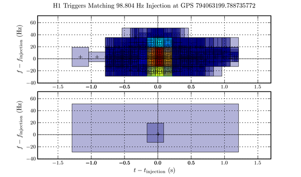
lalapps_power resulting from this one software injection, the bottom panel shows the single trigger in the output of ligolw_bucluster. The large rectangle marks the extent of the triggers that formed the cluster, the small rectangle shows the "most significant portion" of the event, and the small \(+\) marker indicates the time and frequency where it is estimated the burst event's energy peaked (note its proximity to the true centre time and frequency of the injection).The program ligolw_cafe ("coincidence analysis front end") groups trigger files for analysis in the coincidence stage of the pipeline. Normally gravitational wave antennas do not have 100\ particular laser interferometers can frequently "loose lock" so that the time series data recorded from the antenna has gaps in it. This has the side effect of providing natural boundaries in the data on which to divide analysis tasks. For example, if one has a collection of trigger files gathered from two instruments and one wishes to search for coincident events but there are gaps in the times spanned by the files, since events stored in files before a gap cannot be coincident with events stored in files after the gap one can avoid performing unnecessary comparisons in the coincidence analysis by collecting together for coincidence tests only events from within the same continguous group of files. The program ligolw_cafe is used to determine which files need to be grouped together to perform a coincidence analysis among them.
This program takes as input a LAL cache file describing a collection of files to be used in a coincidence analysis. In particular, the instrument and segment columns in the cache file should correctly describe the contents of each file. This program also uses for input a LIGO Light Weight XML file containing a time_slide table describing a list of instrument and time delay combinations to be used in the coincidence analysis. The LAL cache files are named on the command line, or a cache file can be read from stdin. The time slide XML file is specified with a command line option.
The program iteratively applies the time delays from the time_slide table in the time slide XML file to the segments of the files in the input cache. For each time delay and instrument combination, the files whose segments intersect one another are identified and placed together in groups, where the files within a group intersect one another and the files in different groups do not. As different time delay and instrument combinations are considered, the file groups are allowed to coalesce as needed. The final result is a collection of file groups, where no file from one group was ever identified as being coincident with a file from another group in any of the instrument and delay combinations considered. Therefore, the triggers from the files from one group need never be compared to the triggers from the files in another group as it is known in advance that they cannot be coincident.
The output of the program is a collection of LAL cache files, one LAL cache for each coincident group of files that was identified.
One should think of this program as a coincidence analysis applied at the level of entire files, whose role is to reduce the total number of comparisons that need to be performed to complete the full coincidence stage in a pipeline.
The program ligolw_burca actually performs two distinct functions. In the future, it is likely these functions will be split into two applications. The first function performed by this program is an inter-instrument coincidence comparison of the burst events stored in sngl_burst tables in LIGO light-weight XML files. The other function performed by this program is the ranking of \(n\)-tuples of mutually-coincident events according to likelihood ratio data collected from time-slide and injection runs.
The coincidence tests applied by this application are exclusively two-event tests: one event from one instrument is compared to one event from another instrument, and the two are either coincident or not. Events taken from more than two instruments constitute a coincident \(n\)-tuple when they are all pair-wise mutually coincident. Establishing the coincidence of an \(n\)-tuple thus requires \(n\)-choose-2 tests, which scales as \(\order(n^{2})\). The total number of \(n\)-tuples that needs to be tested is, in principle, \(\order(N^{n})\) where \(N\) is the average number of events obtained from each instrument going into the coincidence analysis. A variety of optimization techniques are employed to avoid unnecessary comparisons, but users should not be surprised to find that this program can take a long time to run.
There are two coincidence tests to choose from. These are as follows.
Two events are coincident if their time-frequency tiles are not disjoint after allowing for the light travel time between the two instruments. There are no tunable parameters in this coincidence test, and the light travel times are obtained from an internal look-up table of the locations of known instruments.
When this coincidence test is selected, the output file has a multi_burst table added to it which is populated with summary information about each coincident \(n\)-tuple identified by the coincidence analysis. Each coincident \(n\)-tuple is assigned an SNR equal to the square root of the sum of the squares of the SNRs of the events that participate. Each \(n\)-tuple is also assigned a bandwidth, duration, and peak frequency which are the \(\text{SNR}^{2}\)-weighted averages of the respective quantities from the constituent events. Each \(n\)-tuple is assigned an \(h_{\text{rss}}\) equal to the \(h_{\text{rss}}\) of the most statistically confident of the constituent events, and a confidence equal to the lowest confidence of the constituent events. At the present time, of all of this information only the confidence assigned to the \(n\)-tuple is used elsewhere in the pipeline.
–threshold option from the command line. If the two events are taken from H1 and H2, then in addition to the peak time comparison to be coincident they must also pass an amplitude comparison. Each string cusp burst event has an amplitude \(A\) and an SNR \(\rho\), and the amplitude consistency test requires that \begin{equation} \magnitude{A_{1} - A_{2}} \leq \min \left\{ \magnitude{A_{1}} (\kappa / \rho_{1} + \epsilon), \magnitude{A_{2}} (\kappa / \rho_{2} + \epsilon) \right\}, \end{equation}
where \(\kappa\) and \(\epsilon\) are parameters supplied on the command line.The results of the coincident event search are recorded in coinc tables in the XML files, which are overwritten.
Setting the coincidence test to "<tt>excesspower2</tt>" switches to the likelihood ratio analysis mode. In this mode of operation, ligolw_burca assigns likelihood ratios to the coincident \(n\)-tuples it has previously identified using parameter distribution density data collected from populations of time-slide ("noise") and injection ("gravitational wave") \(n\)-tuples. The procedure goes as follows. First, ligolw_burca is used to identify coincident \(n\)-tuples in time-slide and injection trigger lists. Another program, ligolw_burca_tailor (see this section, scans these \(n\)-tuples and collects summary statistics about their properties. Finally, ligolw_burca is used to reprocess the \(n\)-tuples using the parameter distributions measured by ligolw_burca_tailor to assign likelihood ratio values to each \(n\)-tuple, thereby ranking the \(n\)-tuples from most to least injection-like. Note that typically one will not want to use the same \(n\)-tuples to assign likelihood ratio values to themselves, but this is an unimportant operational detail at this time. See this figure for an example of the \(n\)-tuple parameter distribution functions measured by ligolw_burca_tailor.
Note that in likelihood ratio analysis mode, ligolw_burca processes triggers in SQLite3 database files. Use the program ligolw_sqlite to transform LIGO Light Weight XML files into SQLite3 database files before processing.
The program ligolw_binjfind processes LIGO light weight XML files containing sim_burst, sngl_burst, and optionally coinc_event tables and identifies and records which burst events correspond to injections. There are three kinds of burst/injection matches that are searched for and recorded:
individual burst events in the sngl_burst table that match injections in the sim_burst table,
coincident \(n\)-tuples of burst events that match "exactly" injections in the sim_burst table,
Two burst/injection comparison tests are available, one for use with the excess power burst search pipeline and one for use with the string cusp search pipeline. An "exact" \(n\)-tuple/injection match is one in which every burst event in the coincident \(n\)-tuple is identified as matching the injection according to the burst/injection comparison test. A "nearby" \(n\)-tuple/injection match is a coincident \(n\)-tuple of burst events that occurs within 2 s of the injection (the injection does not precede the first of the events' start times or lag the last of their end times by more than 2 s).
The reason for the two distinct types of \(n\)-tuple/injection matches is that there are two reasons one wishes to identify an injection in a list of burst events. On the one hand, one wishes to characterize the search code in order to measure how well it does or does not recover the parameters of an injection and for this one does not want to be distracted by accidental injection recoveries (when noise in the time series happens to occur near an injection), and so one wishes to identify burst events that really are believed to be the direct result of the software injection. On the other hand, one wishes to measure the detection efficiency of the pipeline or the probability that the pipeline produces a detection candidate when a software injection is placed in the time series. In this case it doesn't matter if the injection is recovered well at all, only whether or not something (anything) survives the pipeline when the injection is placed in the input.
The results of the injection identification tests are recorded in the coinc tables in the XML files, which are overwritten.
The program ligolw_burca_tailor scans the coincident \(n\)-tuples of burst events recorded in LIGO Light Weight XML files and collects statistics on their properties. The resulting parameter distribution densities are written as Array data to LIGO Light Weight XML files which can be used by ligolw_burca to assign likelihood ratio values to coincident \(n\)-tuples.
Note that ligolw_burca_tailor operates on SQLite3 database files. Use the program ligolw_sqlite to transform LIGO Light Weight XML into SQLite3 database files before processing with ligolw_burca_tailor.
This program collects statistics specific to the excess power burst search pipeline. At present, the events in an \(n\)-tuple are taken pair-wise and 5 parameters computed for each pair:
\((\Delta t_{1} - \Delta t_{2}) / \mean{\Delta t}\), the difference in the two events' "most significant" durations as a fraction of the average of the two durations,
\((\Delta f_{1} - \Delta f_{2}) / \mean{\Delta f}\), the difference in the two events' "most significant" bandwidths as a fraction of the average of the two bandwidths,
\((h_{\text{rss}_{1}} - h_{\text{rss}_{2}}) / \mean{h_{\text{rss}}}\), the difference of the two events' \(h_{\text{rss}}\)s as a fraction of the average of the two,
\((f_{1} - f_{2}) / \mean{f}\), the difference of the two events' peak frequencies as a fraction of the average of the two,
The first four quantities are dimensionless and algebraically confined to the interval \([-2, +2]\). The fifth parameter is dimensionful and has no natural interval in which its values are confined. A three-event \(n\)-tuple is characterized by a total of 15 parameters, one set of the five numbers above for each choice of two events from the \(n\)-tuple.
The parameter distributions are tracked by constructing bins, and for each bin counting how many \(n\)-tuples produce a parameter value in the range represented by that bin. When all the \(n\)-tuples have been processed, the bin counts are stored as Array data in an output LIGO Light Weight XML file. For the parameters confined to finite intervals, the distributions are measured using simple linearly-spaced bins. For the \(t_{1} - t_{2}\) parameters a non-linear binning is used in which the bins are uniform in \(\tan^{-1} [(t_{1} - t_{2}) / T]\), where \(T\) is a parameter used to set the scale of the bins. This binning produces bins that are approximately uniformly spaced for small \((t_{1} - t_{2}) / T\), but transition to asymptotically diminishing density for large \((t_{1} - t_{2}) / T\).
this figure shows an example of the parameter distributions measured for time-slide and injection \(n\)-tuples in stationary Gaussian noise.
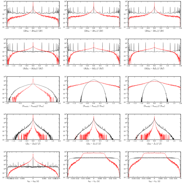
ligolw_burca_tailor. The black curves are the distributions observed in time-slide \(n\)-tuples ("noise"), and the red are the parameter distributions observed in software injection \(n\)-tuples ("gravitational waves").The program ligolw_burca_tailor can also merge LIGO Light Weight XML files containing distribution data into single files. The collection of the statistics can be a time-consuming operation, and it can be convenient to process files in parallel groups on a compute cluster. In this case, it's necessary to be able to merge the bin counts after each group of trigger files has been processed.
Blah blah blah.
The "excess power pipeline" is the search pipeline that results from chaining the programs described above together to perform a multi-instrument search for gravitational wave bursts. Typically the pipeline is executed on a Condor compute cluster (this is the only mode that has been tested). This is done using a set of Condor job control files which instruct Condor as to the sequence of jobs to run and the command line arguments to give each. The Condor control files are generated using a set of Python scripts described below.
Refering to the pipeline schematic in this figure, there are two scripts for building the excess power pipeline. The first script, lalapps_power_pipe, builds the "top half" of the pipeline, the part of the pipeline above the dashed divider in the schematic. This part of the pipeline involves data discovery, optional software injections, trigger identification, clustering, coincidence analysis, and injection identification. The second script, lalapps_power_likelihood_pipe, builds the "bottom half" of the pipeline. In this part of the pipeline, coincident \(n\)-tuple parameter distribution data is used to rank coincidences according to how injection-like they appear.
In the top half of the pipeline, all programs manipulate data files in LIGO Light Weight XML format. In the bottom half, all programs manipulate the data files in SQLite3 database format. The transition from XML to SQLite3 occurs at the end of the top half of the pipeline, where the data processing sequence ends with a set of ligolw_sqlite jobs to convert the files.
The Condor control files for the top and bottom halves of the pipeline can reside in the same directory (there are no name conflicts), so the entire pipeline can be constructed as a pair of DAGs in a single directory.
The Condor control files for the pipeline's top half are constructed using the program lalapps_power_pipe. This program can generate three versions of the pipeline's top half: a version containing the non-injection portion of the pipeline only (the left part of Figure this figure, a version containing the injection portion of the pipeline only (the right part of this figure, or a version containing both injection and non-injection jobs.
To generate the Condor control files, the pipeline construction program lalapps_power_pipe requires the following information as input.
One or more LIGO Light Weight XML files containing one time_slide table each (See ligolw_tisi in this section describing the instrument and time delay combinations to use in the non-injection coincidence stage of the pipeline. These files are not required if the injection-only version of the pipeline is being constructed. Each time slide file results in a separate set of ligolw_burca jobs being constructed. This allows a large number of time slides to be analyzed, distributing them across multiple ligolw_burca jobs.
One LIGO Light Weight XML file containing the time_slide table identifiying the instrument and delay combinations to be used in the injection coincidence stage of the pipeline. This file is not required if the non-injection only version of the pipeline is being constructed. Note that at the present time, the injection stage of the pipeline can only process injections at 0 offset so only all-zero time slides can be given in this input file. However, the instrument combination appearing in the time slides are used to determine which pairs of instruments to combine in the coincidence stage.
A set of files in segwizard format listing the segments to be analyzed. There must be exactly one segment file for each instrument appearing in any of the time slides found in the time slide files.
The pipeline script analyzes the segments and the time slides and determines which time intervals can be analyzed, and which time intervals will be combined together for the coincidence analyses. Instances of lalapps_power are used to generate triggers, and ligolw_bucluster jobs are used to cluster the resulting triggers. The program ligolw_add is used to combine the appropriate trigger files together in preparation for coincidence analysis. At this time, the time slides files generated by the user prior to pipeline construction are also merged into the trigger files, and in the case of the injection branch of the pipeline the list of software injections is also merged into the trigger file. The resulting merged data files are processed with ligolw_burca for coincidence identification, and in the case of the injection portion of the pipeline with ligolw_bucut and ligolw_binjfind to trim the software injection list and identify software injections respectively. Finally, a set of ligolw_sqlite jobs convert the XML files to SQLite3 database files. A representative graph of the parent-child relationships among the jobs is shown in Figure this figure
FIXME: A graph showing the parent-child relationships among the jobs in the top half of the excess power pipeline.
The excess power search identifies time-frequency tiles as events when the probability of getting power in the tile from Gaussian noise alone is below some particular threshold. The search assumes no particular information about the gravitational wave signals other than the time frequency ranges to search for, so once those ranges are chosen the main tool to tune the pipeline is by tweaking the threshold. The other parameter to test in the tuning procedure is the coincidence window. Thus to summarize the parameters to tune in the excess power search are:
In the following sections we will go over the tuning of the different parameters in more details.
The size(duration and bandwidth) of the tiles are largely guided by the time-frequency content of the gravitational waves one is searching for. Here, we describe the tuning procedure where we were concentrating on the search of the merger phase preceded by an inspiral phase. As mentioned before the physical parameters describing the merger phase of a binary black hole coalescence are very poorly understood till today. However there are some rough estimates available in the literature which we will briefly describe here. These will provide us a guideline in choosing the parameters of our search pipeline. [FH:Flannagan and Hughes]
The process of coalescence can be roughly divided into three phases:
The inspiral phase can be modelled accurately enough to use the match filtering techniques to search for the waveforms, however for massive black holes when there are not enough cycles left in the inspiral phase we have to rely on the merger phase for the detection of the coalescence. According to the estimates of FH, binary black hole systems with total mass \(M \leq 30M_{\odot}\) are best searched for via their inspiral waves while systems with \(M > 30M_{\odot}\) must be searched via their merger waves and/or their well understood ringdown waves.
FH has estimated a conservative value for the merger frequency given by
\begin{equation} f_{merge} = \frac{0.02}{M} \\ = 205 Hz (\frac{20M_{\odot}}{M}) \label{eq_fmerge} \end{equation}
. This is conservative in the sense that one can reasonably be sure that numerically generated templates will not be needed before \(f = f_{merger}\). Now LIGO noise floor restricts the lowest frequency that can be searched for and in \(S4\) this is \(\approx 50 Hz\). Using Eq. \eqref{eq_fmerge} we then get that a binary system of maximum mass \(\approx 80M_{\odot}\) can be searched for in \(S4\). However for a \(80 M_{\odot}\) binary the number of cycles in the inspiral phase will be very small and since we are interested in the coincidence of the mergers with the inspirals we would like to restrict our search to a bit lower total mass. Thus the mass range of the binary black holes that we decide to look at for the IB search is given by
\begin{equation} 30 M_{\odot} < M \leq 70 M_{\odot}. \label{eq_massrange} \end{equation}
Given this mass range let us now see what can we estimate about the expected frequency and duration of the merger signals. From Eq. \eqref{eq_fmerge} we get the approximte range of the merger frequencies:
\begin{equation} 58 Hz < f_{merge} \leq 140 Hz \label{eq_frange} \end{equation}
Now according to FH the high frequency shut off for the mergers are roughly given by
\begin{equation} f_{qnr} = 1320 Hz (\frac{20M_{\odot}}{M}) \label{eq_fqnr} \end{equation}
Thus if the assumed bandwidth of the merger signal is \(\Delta f = f_{qnr} - f_{merge}\), then for our mass range of interest we may expect the bandwidth to be of the order of few hundred Hertz.
The effective duration for the signals has also been roughly estimated by FH to be:
\begin{equation} 50 M < T < 10 M \label{eq_timerange} \end{equation}
depending on the total spin of the binary system. If we consider a coalescence where both the inspiraling black holes are nearly maximally spinning, with their spins and the orbital angular momentum nearly alligned then the merger may be expected to be long, while for non-spinning black holes the merger will be rather quick. Thus given our mass range of interest Eq. \eqref{eq_massrange} the time duration of the expected signals whould be somewhere in the range:
\begin{equation} 17.2 ms < T < 1.5 ms \label{eq_trange} \end{equation}
So given these estimates about the bandwidth and the duration of the signals of our main interest we choose the following parameters in our search pipeline:
The last two parameters set the maximum duration and bandwith of a single tile in the search, which does not preclude us from searching for longer or broader signals since we can always sum up the power from multiple tiles triggered by the particular signal.
We saw in this section that the sizes of the tiles are mainly guided by the rough expectations about the signals that we are interested in. However, the threshold on the probability of power in a tile is guided by the optimisation between the false rate and efficiency to a set of Monte Carlo simulations. The idea we usually follow is to choose a threshold which lowers the false rate maintaining the efficiency at an acceptable value.
To get a rough idea about the region where we start loosing significant amount of efficiency without an appreciable effect in lowering the false rate we estimate the efficiencies and the false rates for a number of thresholds. We have used \(Q9\) Sine-Gaussian waveforms at \(235 Hz \) to perform the tuning and the confidence thresholds are \(\{-30.0, -35.0, -40.0, -45.0, -50.0, -55.0, -60.0, -65.0, -70.0, -80.0, -90.0, -100.0, -150.0, -200.0\}\). How the efficiency and the false rate depend on the thresholds are shown in this figure:
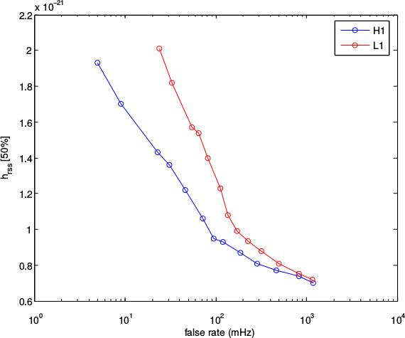
The circles on the curves show the values corresponding to different thresholds. The maximum false rate and the best efficiency are obtained for the lowest |threshold|(30.0), then as the |threshold| is increased the false rate decreases while the efficiency gets worse. Around the |thresholds| of \(50.0 - 60.0\) one may notice that for a very small decrease in false rate the efficiency gets a whole lot worse. This gives us a rough idea that we should choose \( |threshold| < 60.0\). However one should be aware of the fact that tuning must be specific to the pipeline being run. In our pipeline we have a coincidence step which involves the burst triggers and the inspiral triggers and we are not quite sure how many of the false triggers will survive that step. We also plan to use the Hanford 2Km instrument in a coherent follow up at the end of the pipeline which will also hopefully get rid off many of the false triggers. However we would like to have a good estimate of the background distribution of triggers and so have a few surviviors at the end of the pipeline. Keeping that in mind we decided to choose a looser threshold on the confidence probabilities. The thresholds we chose are
These thresholds were so chosen so that the false rate after coincidence between H1 and L1 triggers is \(\approx 2 \) mHz while the \( h_{rss}\) is \(\approx 1.12 \times 10^{-21}\).