|
LALApps 10.1.0.1-8a6b96f
|


|
|
LALApps 10.1.0.1-8a6b96f
|
|

lalapps_inspinj — produces inspiral injection data files.
lalapps_inspinj
[–help] –source-file sfile –mass-file mfile
[–gps-start-time tstart] [–gps-end-time tend]
[–time-step tstep] [–time-interval tinterval]
[–seed seed] [–waveform wave] [–lal-eff-dist] [–usertag tag]
[–tama-output] [–write-eff-dist]
[–ilwd]
lalapps_inspinj generates a number of inspiral parameters suitable for using in a Monte Carlo injection to test the efficiency of a inspiral search. The various parameters (detailed below) are randomly chosen and are appropriate for a particular population of binary neutron stars whose spatial distribution includes the Milky Way and a number of extragalactic objects that are input in a datafile. The possible mass pairs for the binary neutron star com- panions are also specified in a (different) datafile.
The output of this program is a list of the injected events, starting at the specified start time and ending at the specified end time. One injection with random inspiral parameters will be made every specified time step, and will be randomly placed within the specified time interval. The output is written to a file name in the standard inspiral pipeline format:
where USERTAG is tag as specfied on the command line, SEED is the value of the random number seed chosen and GPSSTART and DURATION describes the GPS time interval that the file covers. The file is in the standard LIGO lightweight XML format containing a sim_inspiral table that describes the injections. In addition, an ASCII log file called injlog.txt is also written. If a –user-tag is not specified on the command line, the _USERTAG part of the filename will be omitted.
–help: Print a help message.
–source-file sfile: Optional. Data file containing spatial distribution of extragalactic objects. Default is the file inspsrcs.dat provided by LALApps. If that file is empty, all signals are in the Milky Way.
–mass-file mfile: Optional. Data file containing mass pairs for the binary neutron star companions. Default is the file BNSMasses.dat provided by LALApps.
–gps-start-time tstart: Optional. Start time of the injection data to be created. Defaults to the start of S2, Feb 14 2003 16:00:00 UTC (GPS time 729273613)
–gps-end-time tend: Optional. End time of the injection data to be created. Defaults to the end of S2, Apr 14 2003 15:00:00 UTC (GPS time 734367613).
–time-step tstep: Optional. Sets the time step interval between injections. The injections will occur with an average spacing of tstep seconds. Defaults to \(2630/\pi\).
–time-interval tinterval: Optional. Sets the time interval during which an injection can occur. Injections are uniformly distributed over the interval. Setting tstep to \(6370\) and tinterval to 600 guarantees there will be one injection into each playground segment and they will be randomly distributed within the playground times - taken the fact that your gps start time coincides with start of a playground segment.
–seed seed: Optional. Seed the random number generator with the integer seed. Defaults to \(1\).
–waveform wave: Optional. The string wave will be written into the waveform column of the sim_inspiral table output. This is used by the inspiral code to determine which type of waveforms it should inject into the data. Defaults is GeneratePPNtwoPN.
–lal-eff-dist: Optional. If this option is specified, the effective distance will be calculated using routines from LAL. Otherwise, the default behaviour is to use an independent method contained in inspinj.c. There is good agreement between these two methods, see below for more details.
–user-tag string: Optional. Set the user tag for this job to be string. May also be specified on the command line as -userTag for LIGO database compatibility.
–tama-output: Optional. If this option is given, lalapps_inspinj also produces a text output file:
which contains the following fields:
In the above, all times are recorded as double precision real numbers and all angles are in radians. The TAMA polarization is calculated using
\begin{equation} \tan( \psi_{T} ) = \frac{ x \cdot T_{z} }{ y \cdot T_{z} } \, . \end{equation}
Here x and y are the x,y axes of the radiation frame expressed in earth fixed coordinates Eq. \eqref{xrad}, Eq. \eqref{yrad}. \(T_{z}\) is a unit vector in earth fixed coordinates which is orthogonal to the two arms of the TAMA detector Eq. \eqref{tarm}. It is given by
\begin{equation} T_{z} = ( -0.6180, +0.5272, +0.5832 ) \end{equation}
–write-eff-dist: Optional. If this option is given, three extra columns are added to the TAMA output file described above. They are
These entries are added to the list immediately after TAMA end time and before total mass.
–ilwd: Optional. If this option is given, lalapps_inspinj also produces two ILWD-format files, injepochs.ilwd and injparams.ilwd, that contain, respectively, the GPS times suitable for inspiral injections, and the intrinsic inspiral signal parameters to be used for those injections.
The file injepochs.ilwd contains a sequence of integer pairs representing the injection GPS time in seconds and residual nano-seconds. The file injparams.ilwd contains the intrinsic binary parameters for each injection, which is a sequence of eight real numbers representing (in order) (1) the total mass of the binary system (in solar masses), (2) the dimensionless reduced mass — reduced mass per unit total mass — in the range from 0 (extreme mass ratio) to 0.25 (equal masses), (3) the distance to the system in meters, (4) the inclination of the binary system orbit to the plane of the sky in radians, (5) the coalescence phase in radians, (6) the longitude to the direction of the source in radians, (7) the latitude to the direction of the source in radians, (8) and the polar- ization angle of the source in radians.
The algorithm for computing the effective distance will be described in some detail below. The method is to compute both the strain due to the inspiral and the detector response in the earth fixed frame. This frame is such that the z-axis points from the earth's centre to the North Pole, the x-axis points from the centre to the intersection of the equator and the prime meridian and the y-axis is chosen to complete the orthonormal basis. The coordinates of the injection are specified by longitude (or right ascension) \(\alpha\) and latitude (or declination) \(\delta\). The polarization is appropriate for transferring from the radiation to earth fixed frame. These are then converted to the earth fixed frame by
\begin{eqnarray} \theta &=& \frac{\pi}{2} - \delta \\ \phi &=& \alpha - \textrm{gmst} \, . \end{eqnarray}
Here, gmst is the Greenwich Mean sidereal time of the injection. The axes of the radiation frame (x,y,z) can be expressed in terms of the earth fixed coordinates as:
\begin{eqnarray} x(1) &=& +( \sin( \phi ) \cos( \psi ) - \sin( \psi ) \cos( \phi ) \cos( \theta ) ) \nonumber \\ x(2) &=& -( \cos( \phi ) \cos( \psi ) + \sin( \psi ) \sin( \phi ) \cos( \theta ) ) \nonumber \\ x(3) &=& \sin( \psi ) \sin( \theta ) \label{xrad}\\ y(1) &=& -( \sin( \phi ) \sin( \psi ) + \cos( \psi ) \cos( \phi ) \cos( \theta ) ) \nonumber\\ y(2) &=& +( \cos( \phi ) \sin( \psi ) - \cos( \psi ) \sin( \phi ) \cos( \theta ) ) \nonumber \\ y(3) &=& \cos( \psi ) \sin( \theta ) \label{yrad} \end{eqnarray}
Making use of these expressions, we can express the gravitational wave strain in earth fixed coordinates as
\begin{equation}\label{hij} h_{ij} = ( h^{+}(t) e^{+}_{ij} ) + (h^{\times}(t) e^{\times}_{ij}) \end{equation}
where
\begin{equation} e^{+}_{ij} = x_{i} * x_{j} - y_{i} * y_{j} \qquad \mathrm{and} \qquad e^{\times}_{ij} = x_{i} * y_{j} + y_{i} * x_{j}. \end{equation}
For the case of a binary inspiral signal, the two polarizations \(h^{+}\) and \(h^{\times}\) of the gravitational wave are given by
\begin{eqnarray} h^{+}(t) &=& \frac{A}{r} ( 1 + \cos^2 ( \iota ) ) * \cos( \Phi(t) ) \\ h^{\times}(t) &=& \frac{A}{r} * ( 2 \cos( \iota ) ) * \sin( \Phi(t) ) \end{eqnarray}
where \(A\) is a mass and frequency dependent amplitude factor, \(r\) is the physical distance at which the injection is located and \(\iota\) is the inclination angle.
Next, we can write the detector response function as
\begin{equation} d^{ij} = \left(\frac{1}{2} \right) \left( n_{x}^{i} n_{x}^{j} - n_{y}^{i} n_{y}^{j} \right) \, . \end{equation}
Here, \(n_{x}\) and \(n_{y}\) are unit vectors directed along the arms of the detector. Specifically, for the Hanford, Livingston, GEO, TAMA and Virgo detectors we use:
\begin{eqnarray} H_{x} &=& ( -0.2239, +0.7998, +0.5569 ) \nonumber \\ H_{y} &=& ( -0.9140, +0.0261, -0.4049 ) \\ L_{x} &=& ( -0.9546, -0.1416, -0.2622 ) \nonumber \\ L_{y} &=& ( +0.2977, -0.4879, -0.8205 ) \\ G_{x} &=& ( -0.6261, -0.5522, +0.5506 ) \nonumber \\ G_{y} &=& ( -0.4453, +0.8665, +0.2255 ) \\ T_{x} &=& ( +0.6490, +0.7608, +0.0000 ) \nonumber \\ T_{y} &=& ( -0.4437, +0.3785, -0.8123 ) \label{tarm} \\ V_{x} &=& ( -0.7005, +0.2085, +0.6826 ) \nonumber \\ V_{y} &=& ( -0.0538, -0.9691, +0.2408 ) \end{eqnarray}
The response of an interferometric detector with arm locations given by \(n_{x}\) and \(n_{y}\) to an inspiralling binary system described by Eq. \eqref{hij} is
\begin{eqnarray} h(t) &=& h^{+}(t) ( d^{ij} e^{+}_{ij} ) + h^{\times}(t) ( d^{ij} e^{\times}_{ij} ) \nonumber \\ &=& \left(\frac{A}{r}\right) \left[ ( 1 + \cos^2 ( \iota ) ) F_{+} \cos( \Phi(t)) + 2 \cos( \iota ) F_{\times} \sin( \Phi(t) ) \right] \, , \end{eqnarray}
where we have introduced
\begin{equation} F_{+} = d^{ij} e^{+}_{ij} \qquad \mathrm{and} \qquad F_{\times} = d^{ij} e^{\times}_{ij} \end{equation}
Finally, to calculate the effective distance, we note that the two contributions to \(h(t)\) are \(\pi/2\) radians out of phase, and hence orthogonal. Thus, we can compute the effective distance to be:
\begin{equation} D_{\mathrm{eff}} = r / \left( \frac{ (1 + \cos^2(\iota))^2 }{4} F_{+}^{2} + cos^{2}(\iota) F_{\times}^{2} \right) \end{equation}
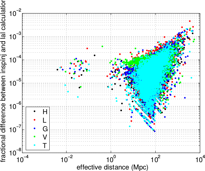
The algorithm to calculate effective distances described above is completely contained within inspinj.c. There is an independent method of computing effective distances can also be called by inspinj. It is contained in the LAL function LALPopulateSimInspiralSiteInfo(). This function populates the site end time and effective distance for all the interferomter sites. It makes use of LAL functionality in the tools and date packages. These same functions are used when generating the injection waveform which is added to the data stream (in lalapps_inspiral). As a check that these two calculations produce the same effective distance, lalapps_inspinj was run twice, once with the –lal-eff-dist option and once without. This figure shows the fractional difference in effective distance between the two methods for a set of injections. We see that the distances agree within 1\ occuring for the largest effective disances, i.e. close to the dead spot of the instrument. For injections which initial LIGO is sensitive to, the accuracy is few \(\times 10^{-4}\).
BNSMasses.dat and the default source file inspsrcs.dat. Definition in file inspinj.c.
Go to the source code of this file.
Data Structures | |
| struct | FakeGalaxy |
Macros | |
| #define | CVS_REVISION "$Revision$" |
| #define | CVS_ID_STRING "$Id$" |
| #define | CVS_SOURCE "$Source$" |
| #define | CVS_DATE "$Date$" |
| #define | CVS_NAME_STRING "$Name$" |
| #define | PROGRAM_NAME "inspinj" |
| #define | ADD_PROCESS_PARAM(pptype, format, ppvalue) |
| #define | AXIS_MAX 12 |
| #define ADD_PROCESS_PARAM | ( | pptype, | |
| format, | |||
| ppvalue | |||
| ) |
| void drawLocationFromExttrig | ( | SimInspiralTable * | table | ) |
| void drawMassFromSource | ( | SimInspiralTable * | table | ) |
| void drawMassSpinFromNR | ( | SimInspiralTable * | table | ) |
| void drawMassSpinFromNRNinja2 | ( | SimInspiralTable * | table | ) |
| void adjust_snr | ( | SimInspiralTable * | inj, |
| REAL8 | target_snr, | ||
| const char * | ifos | ||
| ) |
| void adjust_snr_real8 | ( | SimInspiralTable * | inj, |
| REAL8 | target_snr, | ||
| const char * | ifos | ||
| ) |
| REAL8 network_snr | ( | const char * | ifos, |
| SimInspiralTable * | inj | ||
| ) |
| REAL8 snr_in_ifo | ( | const char * | ifo, |
| SimInspiralTable * | inj | ||
| ) |
| REAL8 network_snr_real8 | ( | const char * | ifos, |
| SimInspiralTable * | inj | ||
| ) |
| REAL8 snr_in_ifo_real8 | ( | const char * | ifo, |
| SimInspiralTable * | inj | ||
| ) |
| REAL8 snr_in_psd_real8 | ( | const char * | ifo, |
| REAL8FrequencySeries * | psd, | ||
| REAL8 | start_freq, | ||
| SimInspiralTable * | inj | ||
| ) |
| REAL8 network_snr_with_psds_real8 | ( | int | num_ifos, |
| const char ** | ifo_list, | ||
| REAL8FrequencySeries ** | psds, | ||
| REAL8 * | start_freqs, | ||
| SimInspiralTable * | inj | ||
| ) |
| void adjust_snr_with_psds_real8 | ( | SimInspiralTable * | inj, |
| REAL8 | target_snr, | ||
| int | num_ifos, | ||
| const char ** | ifo_list, | ||
| REAL8FrequencySeries ** | psds, | ||
| REAL8 * | start_freqs | ||
| ) |
|
static |
|
extern |
defined in lal/lib/std/LALError.c
| LoudnessDistribution dDistr |
| SkyLocationDistribution lDistr |
| MassDistribution mDistr |
| InclDistribution iDistr |
| SpinDistribution spinDistr = uniformSpinDist |
| SimInspiralTable* simTable |
| SimRingdownTable* simRingTable |
| AlignmentType alignInj = notAligned |
|
static |
| ExtTriggerTable* exttrigHead = NULL |
| char name[LIGOMETA_SOURCE_MAX] |
| struct { ... } * source_data |
| struct { ... } * old_source_data |
| struct { ... } * temparray |
| struct { ... } * skyPoints |
| char MW_name[LIGOMETA_SOURCE_MAX] = "MW" |
| struct { ... } * mass_data |
| LIGOTimeGPS* inj_times |
| SimInspiralTable** nrSimArray = NULL |