|
LALPulsar 7.1.1.1-2c25347
|


|
|
LALPulsar 7.1.1.1-2c25347
|
|

Provides routines to generate continuous waveforms with spindown and orbital modulation.
This header covers routines to generate continuous quasiperiodic waveforms with a smoothly-varying intrinsic frequency modulated by orbital motions around a binary companion. The intrinsic frequency is modeled by Taylor series coefficients as in GenerateTaylorCW.h, and the orbital modulation is described by a reduced set of orbital parameters. Note that the routines do not account for spin precession, accretion processes, or other complicating factors; they simply Doppler-modulate a polynomial frequency function.
The frequency and phase of the wave in the source's rest frame are given by Eq. \eqref{eq_taylorcw-freq} and Eq. \eqref{eq_taylorcw-phi} of Header GenerateTaylorCW.h, where \( t \) is the proper time in this rest frame. The frequency and phase of the wave fronts crossing a reference point in an inertial frame (e.g. the Solar system barycentre) are simply \( f[t(t_r)] \) and \( \phi[t(t_r)] \) , where
\begin{equation} \label{eq_spinorbit-tr} t_r = t + R(t)/c \end{equation}
is the (retarded) time measured at the inertial reference point a distance \( r \) from the source.
The generation of the waveform thus consists of computing the radial component \( R(t) \) of the orbital motion of the source in the binary centre-of-mass frame, inverting Eq. \eqref{eq_spinorbit-tr} to find the "emission time" \( t \) for a given "detector time" \( t_r \) , and plugging this into the Taylor expansions to generate the instantaneous frequency and phase. The received frequency is also multiplied by the instantaneous Doppler shift \( [1+\dot{R}(t)/c]^{-1} \) at the time of emission.
Since we do not include precession effects, the polarization state of the wave is constant: we simply specify the polarization amplitudes \( A_+ \) , \( A_\times \) and the polarization phase \( \psi \) based on the (constant) orientation of the source's rotation. The following discussion defines a set of parameters for the source's orbital revolution, which we regard as completely independent from its rotation.
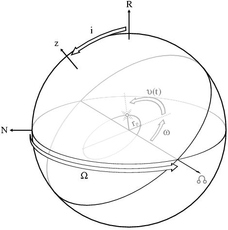
this figure illustrates the notation conventions defining a binary orbit. We define a radial axis \( R \) directed from the observer (Earth) to the source, as shown. The horizontal plane is thus the plane of the sky, and the direction marked \( N \) is the direction along a meridian towards the North celestial pole. The tilted plane is the plane of the binary orbit, and the axis labeled \( z \) is the normal to this plane directed such that the orbit is right-handed about this axis. The ascending node of the orbit, denoted by ☊, is the direction defined by \( \hat{\mathbf{\mathit{R}}}\times\hat{\mathbf{\mathit{z}}} \) . The binary orbit itself is shown as an off-centred ellipse, with the barycentre at one of its foci; the wave-emitting source is also shown.
The inclination angle \( i \) is the angle between the sky and orbital planes. The longitude of the ascending node \( \Omega \) is the angle in the plane of the sky from the North direction to the ascending node, measured right-handed about \( \hat{\mathbf{\mathit{R}}} \) . The argument of the periapsis \( \omega \) is the angle in the orbital plane from the ascending node to the direction of periapsis (point where the source is closest to the system barycentre), and the true anomaly \( \upsilon(t) \) of the source is the angle from the periapsis to the current location of the source; both angles are measured right-handed about \( \hat{\mathbf{\mathit{z}}} \) (i.e. prograde). The periapsis separation \( r_p \) is the distance from the periapsis to the barycentre, and we denote the eccentricity of the orbital ellipse as \( e \) , so that the separation between the source and the barycentre at any time is \( r=r_p(1+e)/(1+e\cos\upsilon) \) .
In this convention, \( i\in[0,\pi] \) and \( \Omega\in[0,2\pi) \) . Another convention common in astronomy is to restrict \( \Omega \) to the range \( [0,\pi) \) , refering to whichever node (ascending or descending) lies in this range. The argument of the periapsis \( \omega \) is then also measured from this node. In this case the range of \( i \) must be extended to \( (-\pi,\pi] \) ; it is negative if the reference node is descending, and positive if it is ascending. The formulae that follow are the same in either convention, though, since one can verify that adding \( \pi \) to \( \Omega \) and \( \omega \) is equivalent to reversing the sign on \( i \) .
Some spherical trigonometry gives us \( R=r\sin(\omega+\upsilon)\sin i \) . We can differentiate \( R \) with respect to \( t \) , and apply Keplers second law \( r^2\dot{\upsilon}=r_p^2\dot{\upsilon}_p=\mathrm{constant} \) , where \( \dot{\upsilon}_p \) is the angular speed at periapsis, to get:
\begin{eqnarray} \label{eq_orbit-r} R & = & R_0 + \frac{(1+e) r_p\sin i}{1+e\cos\upsilon} \sin(\omega+\upsilon) \;,\\ \label{eq_orbit-rdot} \dot{R} & = & \dot{R}_0 + \frac{\dot{\upsilon}_p r_p\sin i}{1+e} \left[ \cos(\omega+\upsilon) + e\cos\omega \right] \;. \end{eqnarray}
Without loss of generality, we will henceforth drop the offsets \( R_0 \) and (constant) \( \dot{R}_0 \) from these equations. This means that we ignore the overall propagation delay between the \( R=R_0 \) plane and the observer, and incorporate any (constant) Doppler shifts due to net centre-of-mass motions into the values of \( f \) and \( \dot{\upsilon}_p \) . The resulting times and parameter values are referred to as being in the barycentric frame. The only time delays and Doppler shifts that we explicitly treat are those arising from the motion of the source relative to the \( R=R_0 \) sky plane passing through the system barycentre.
All we need now to determine the orbital motion is an equation for \( \upsilon(t) \) . Many basic astronomy textbooks give exact but transcendental expressions relating \( \upsilon \) and \( t \) for elliptical orbits with \( 0\leq e<1 \) , and/or series expansions of \( \upsilon(t) \) for \( e\ll1 \) . However, for a generic binary system we cannot guarantee that \( e\ll1 \) , and for now we would like to retain the possibility of modeling open orbits with \( e\geq1 \) . For now we will simply present the exact formulae, and discuss the numerical solution methods in the modules under this header.
Let \( t_p \) be the time of a periapsis passage (preferably a recent one in the case of closed orbits). We express both \( t \) and \( \upsilon \) in terms of an intermediate variable \( E \) (called the eccentric anomaly for elliptic orbits, unnamed for open orbits). The formulae are:
\begin{equation} \label{eq_spinorbit-t} t - t_p = \left\{ \begin{array}{l@{\qquad}c} \frac{1}{\dot{\upsilon}_p} \sqrt{\frac{1+e}{(1-e)^3}} \left( E - e\sin E \right) & 0 \leq e < 1 \\ & \\ \frac{1}{\dot{\upsilon}_p} E \left( 1 + \frac{E^2}{12} \right) & e = 1 \\ & \\ \frac{1}{\dot{\upsilon}_p} \sqrt{\frac{e+1}{(e-1)^3}} \left( e\sinh E - E \right) & e > 1 \end{array} \right. \end{equation}
\begin{equation} \label{eq_spinorbit-upsilon} \begin{array}{c} \tan\left(\frac{\upsilon}{2}\right) \end{array} = \left\{ \begin{array}{l@{\qquad}c} \sqrt{\frac{1+e}{1-e}}\tan\left(\frac{E}{2}\right) & 0 \leq e < 1 \\ & \\ \frac{E}{2} & e = 1 \\ & \\ \sqrt{\frac{e+1}{e-1}}\tanh\left(\frac{E}{2}\right) & e > 1 \end{array} \right. \end{equation}
Thus to solve for \( \upsilon(t) \) one typically inverts the equation for \( t-t_p \) numerically or by series expansion, finds the corresponding \( E \) , and then plugs this into the expression for \( \upsilon \) . However, in our case we would then need to do another numerical inversion to find the retarded time \( t_r \) from Eq. \eqref{eq_spinorbit-tr}. A more efficient approach is thus to take an initial guess for \( E \) , compute both \( t \) , \( \upsilon \) , and hence \( t_r \) , and then refine directly on \( E \) .
Since we may deal with highly eccentric or open orbits, we will specify these orbits with parameters that are definable for all classes of orbit. Thus we specify the size of the orbit with the periapsis separation \( r_p \) rather than the semimajor axis \( a \) , and the speed of the orbit with the angular speed at periapsis \( \dot{\upsilon}_p \) rather than with the period \( P \) . These parameters are related by:
\begin{eqnarray} \label{eq_spinorbit-a} a & = & \frac{r_p}{1-e} \;,\\ \label{eq_spinorbit-p} P & = & \frac{2\pi}{\dot{\upsilon}_p} \sqrt{\frac{1+e}{(1-e)^3}} \;. \end{eqnarray}
Furthermore, for improved numerical precision when dealing with near-parabolic orbits, we specify the value of \( 1-e \) rather than the value of \( e \) . We note that \( 1-e \) has a maximum value of \( 1 \) for a circular orbit, positive for closed elliptical orbits, zero for parabolic orbits, and negative (unbounded) for hyperbolic orbits.
Prototypes | |
| int | XLALGenerateSpinOrbitCW (PulsarCoherentGW *sourceSignal, SpinOrbitCWParamStruc *sourceParams) |
| FIXME: Temporary XLAL-wapper to LAL-function LALGenerateSpinOrbitCW() More... | |
| void | LALGenerateSpinOrbitCW (LALStatus *, PulsarCoherentGW *output, SpinOrbitCWParamStruc *params) |
| Computes a spindown- and Doppler-modulated continuous waveform. More... | |
| void | LALGenerateEllipticSpinOrbitCW (LALStatus *, PulsarCoherentGW *output, SpinOrbitCWParamStruc *params) |
| Computes a continuous waveform with frequency drift and Doppler modulation from an elliptical orbital trajectory. More... | |
| void | LALGenerateParabolicSpinOrbitCW (LALStatus *, PulsarCoherentGW *output, SpinOrbitCWParamStruc *params) |
| Computes a continuous waveform with frequency drift and Doppler modulation from a parabolic orbital trajectory. More... | |
| void | LALGenerateHyperbolicSpinOrbitCW (LALStatus *, PulsarCoherentGW *output, SpinOrbitCWParamStruc *params) |
| Computes a continuous waveform with frequency drift and Doppler modulation from a hyperbolic orbital trajectory. More... | |
Data Structures | |
| struct | SpinOrbitCWParamStruc |
| This structure stores the parameters for constructing a gravitational waveform with both a Taylor-polynomial intrinsic frequency and phase, and a binary-orbit modulation. More... | |
Error Codes | |
| #define | GENERATESPINORBITCWH_ENUL 1 |
| Unexpected null pointer in arguments. More... | |
| #define | GENERATESPINORBITCWH_EOUT 2 |
| Output field a, f, phi, or shift already exists. More... | |
| #define | GENERATESPINORBITCWH_EMEM 3 |
| Out of memory. More... | |
| #define | GENERATESPINORBITCWH_EECC 4 |
| Eccentricity out of range. More... | |
| #define | GENERATESPINORBITCWH_EFTL 5 |
| Periapsis motion is faster than light. More... | |
| #define | GENERATESPINORBITCWH_ESGN 6 |
| Sign error: positive parameter expected. More... | |
| int XLALGenerateSpinOrbitCW | ( | PulsarCoherentGW * | sourceSignal, |
| SpinOrbitCWParamStruc * | sourceParams | ||
| ) |
FIXME: Temporary XLAL-wapper to LAL-function LALGenerateSpinOrbitCW()
NOTE: This violates the current version of the XLAL-spec, but is unavoidable at this time, as LALGenerateSpinOrbitCW() hasn't been properly XLALified yet, and doing this would be beyond the scope of this patch. However, doing it here in this way is better than calling LALGenerateSpinOrbitCW() from various far-flung XLAL-functions, as in this way the "violation" is localized in one place, and serves as a reminder for future XLAL-ification at the same time.
| [out] | sourceSignal | output signal |
| [in] | sourceParams | input parameters |
Definition at line 41 of file GenerateSpinOrbitCW.c.
| void LALGenerateSpinOrbitCW | ( | LALStatus * | stat, |
| PulsarCoherentGW * | output, | ||
| SpinOrbitCWParamStruc * | params | ||
| ) |
Computes a spindown- and Doppler-modulated continuous waveform.
This function computes a quasiperiodic waveform using the spindown and orbital parameters in *params, storing the result in *output.
In the *params structure, the routine uses all the "input" fields specified in Header GenerateSpinOrbitCW.h, and sets all of the "output" fields. If params->f=NULL, no spindown modulation is performed. If params->rPeriNorm=0, no Doppler modulation is performed.
In the *output structure, the field output->h is ignored, but all other pointer fields must be set to NULL. The function will create and allocate space for output->a, output->f, and output->phi as necessary. The output->shift field will remain set to NULL.
This routine calls LALGenerateCircularSpinOrbitCW(), LALGenerateCircularSpinOrbitCW(), LALGenerateCircularSpinOrbitCW(), or LALGenerateCircularSpinOrbitCW(), depending on the value of params->oneMinusEcc. See the other modules under Header GenerateSpinOrbitCW.h for descriptions of these routines' algorithms.
If params->rPeriNorm=0, this routine will call LALGenerateTaylorCW() to generate the waveform. It creates a TaylorCWParamStruc from the values in *params, adjusting the values of params->phi0, params->f0, and params->f from the reference time params->spinEpoch to the time params->epoch, as follows: Let \( \Delta
t=t^{(2)}-t^{(1)} \) be the time between the old epoch \( t^{(1)} \) and the new one \( t^{(2)} \) . Then the phase, base frequency, and spindown parameters for the new epoch are:
\begin{eqnarray} \phi_0^{(2)} & = & \phi_0^{(1)} + 2\pi f_0^{(1)}t \left( 1 + \sum_{k=1}^N \frac{1}{k+1}f_k^{(1)} \Delta t^k \right) \\ f_0^{(2)} & = & f_0^{(1)} \left( 1 + \sum_{k=1}^N f_k^{(1)} \Delta t^k \right) \\ f_k^{(2)} & = & \frac{f_0^{(1)}}{f_0^{(2)}} \left( f_k^{(1)} + \sum_{j=k+1}{N} \binom{j}{k} f_j^{(1)}\Delta t^{j-k} \right) \end{eqnarray}
The phase function \( \phi(t)=\phi_0^{(i)}+2\pi f_0^{(i)}\left[t-t^{(i)}+\sum_{k=1}^N \frac{f_k^{(i)}}{k+1}\left(t-t^{(i)}\right)^{k+1}\right] \) then has the same functional dependence on \( t \) for either \( i=1 \) or~2.
Definition at line 131 of file GenerateSpinOrbitCW.c.
| void LALGenerateEllipticSpinOrbitCW | ( | LALStatus * | stat, |
| PulsarCoherentGW * | output, | ||
| SpinOrbitCWParamStruc * | params | ||
| ) |
Computes a continuous waveform with frequency drift and Doppler modulation from an elliptical orbital trajectory.
This function computes a quaiperiodic waveform using the spindown and orbital parameters in *params, storing the result in *output.
In the *params structure, the routine uses all the "input" fields specified in Header GenerateSpinOrbitCW.h, and sets all of the "output" fields. If params->f=NULL, no spindown modulation is performed. If params->oneMinusEcc \( \notin(0,1] \) (an open orbit), or if params->rPeriNorm \( \times \) params->angularSpeed \( \geq1 \) (faster-than-light speed at periapsis), an error is returned.
In the *output structure, the field output->h is ignored, but all other pointer fields must be set to NULL. The function will create and allocate space for output->a, output->f, and output->phi as necessary. The output->shift field will remain set to NULL.
For elliptical orbits, we combine Eq. \eqref{eq_spinorbit-tr}, Eq. \eqref{eq_spinorbit-t}, and Eq. \eqref{eq_spinorbit-upsilon} to get \( t_r \) directly as a function of the eccentric anomaly \( E \) :
\begin{eqnarray} \label{eq_tr-e1} t_r = t_p & + & \left(\frac{r_p \sin i}{c}\right)\sin\omega\\ & + & \left(\frac{P}{2\pi}\right) \left( E + \left[v_p(1-e)\cos\omega - e\right]\sin E + \left[v_p\sqrt{\frac{1-e}{1+e}}\sin\omega\right] [\cos E - 1]\right) \;, \end{eqnarray}
where \( v_p=r_p\dot{\upsilon}_p\sin i/c \) is a normalized velocity at periapsis and \( P=2\pi\sqrt{(1+e)/(1-e)^3}/\dot{\upsilon}_p \) is the period of the orbit. For simplicity we write this as:
\begin{equation} \label{eq_tr-e2} t_r = T_p + \frac{1}{n}\left( E + A\sin E + B[\cos E - 1] \right) \;, \end{equation}
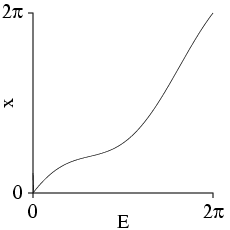
where \( T_p \) is the observed time of periapsis passage and \( n=2\pi/P \) is the mean angular speed around the orbit. Thus the key numerical procedure in this routine is to invert the expression \( x=E+A\sin E+B(\cos E - 1) \) to get \( E(x) \) . We note that \( E(x+2n\pi)=E(x)+2n\pi \) , so we only need to solve this expression in the interval \( [0,2\pi) \) , sketched to the right.
We further note that \( A^2+B^2<1 \) , although it approaches 1 when \( e\rightarrow1 \) , or when \( v_p\rightarrow1 \) and either \( e=0 \) or \( \omega=\pi \) . Except in this limit, Newton-Raphson methods will converge rapidly for any initial guess. In this limit, though, the slope \( dx/dE \) approaches zero at the point of inflection, and an initial guess or iteration landing near this point will send the next iteration off to unacceptably large or small values. However, by restricting all initial guesses and iterations to the domain \( E\in[0,2\pi) \) , one will always end up on a trajectory branch that will converge uniformly. This should converge faster than the more generically robust technique of bisection. (Note: the danger with Newton's method has been found to be unstable for certain binary orbital parameters. So if Newton's method fails to converge, a bisection algorithm is employed.)
In this algorithm, we start the computation with an arbitrary initial guess of \( E=0 \) , and refine it until the we get agreement to within 0.01 parts in part in \( N_\mathrm{cyc} \) (where \( N_\mathrm{cyc} \) is the larger of the number of wave cycles in an orbital period, or the number of wave cycles in the entire waveform being generated), or one part in \( 10^{15} \) (an order of magnitude off the best precision possible with REAL8 numbers). The latter case indicates that REAL8 precision may fail to give accurate phasing, and one should consider modeling the orbit as a set of Taylor frequency coefficients \'{a} la LALGenerateTaylorCW(). On subsequent timesteps, we use the previous timestep as an initial guess, which is good so long as the timesteps are much smaller than an orbital period. This sequence of guesses will have to readjust itself once every orbit (as \( E \) jumps from \( 2\pi \) down to 0), but this is relatively infrequent; we don't bother trying to smooth this out because the additional tests would probably slow down the algorithm overall.
Once a value of \( E \) is found for a given timestep in the output series, we compute the system time \( t \) via Eq. \eqref{eq_spinorbit-t}, and use it to determine the wave phase and (non-Doppler-shifted) frequency via Eq. \eqref{eq_taylorcw-freq} and Eq. \eqref{eq_taylorcw-phi}. The Doppler shift on the frequency is then computed using Eq. \eqref{eq_spinorbit-upsilon} and Eq. \eqref{eq_orbit-rdot}. We use \( \upsilon \) as an intermediate in the Doppler shift calculations, since expressing \( \dot{R} \) directly in terms of \( E \) results in expression of the form \( (1-e)/(1-e\cos E) \) , which are difficult to simplify and face precision losses when \( E\sim0 \) and \( e\rightarrow1 \) . By contrast, solving for \( \upsilon \) is numerically stable provided that the system atan2() function is well-designed.
The routine does not account for variations in special relativistic or gravitational time dilation due to the elliptical orbit, nor does it deal with other gravitational effects such as Shapiro delay. To a very rough approximation, the amount of phase error induced by gravitational redshift goes something like \( \Delta\phi\sim fT(v/c)^2\Delta(r_p/r) \) , where \( f \) is the typical wave frequency, \( T \) is either the length of data or the orbital period (whichever is smaller), \( v \) is the true (unprojected) speed at periapsis, and \( \Delta(r_p/r) \) is the total range swept out by the quantity \( r_p/r \) over the course of the observation. Other relativistic effects such as special relativistic time dilation are comparable in magnitude. We make a crude estimate of when this is significant by noting that \( v/c\gtrsim v_p \) but \( \Delta(r_p/r)\lesssim 2e/(1+e) \) ; we take these approximations as equalities and require that \( \Delta\phi\lesssim\pi \) , giving:
\begin{equation} \label{eq_relativistic-orbit} f_0Tv_p^2\frac{4e}{1+e}\lesssim1 \;. \end{equation}
When this critereon is violated, a warning is generated. Furthermore, as noted earlier, when \( v_p\geq1 \) the routine will return an error, as faster-than-light speeds can cause the emission and reception times to be non-monotonic functions of one another.
Definition at line 169 of file GenerateEllipticSpinOrbitCW.c.
| void LALGenerateParabolicSpinOrbitCW | ( | LALStatus * | stat, |
| PulsarCoherentGW * | output, | ||
| SpinOrbitCWParamStruc * | params | ||
| ) |
Computes a continuous waveform with frequency drift and Doppler modulation from a parabolic orbital trajectory.
This function computes a quaiperiodic waveform using the spindown and orbital parameters in *params, storing the result in *output.
In the *params structure, the routine uses all the "input" fields specified in Header GenerateSpinOrbitCW.h, and sets all of the "output" fields. If params->f=NULL, no spindown modulation is performed. If params->oneMinusEcc \( \neq0 \) , or if params->rPeriNorm \( \times \) params->angularSpeed \( \geq1 \) (faster-than-light speed at periapsis), an error is returned.
In the *output structure, the field output->h is ignored, but all other pointer fields must be set to NULL. The function will create and allocate space for output->a, output->f, and output->phi as necessary. The output->shift field will remain set to NULL.
For parabolic orbits, we combine Eq. \eqref{eq_spinorbit-tr}, Eq. \eqref{eq_spinorbit-t}, and Eq. \eqref{eq_spinorbit-upsilon} to get \( t_r \) directly as a function of \( E \) :
\begin{equation} \label{eq_cubic-e} t_r = t_p + \frac{r_p\sin i}{c} \left[ \cos\omega + \left(\frac{1}{v_p} + \cos\omega\right)E - \frac{\sin\omega}{4}E^2 + \frac{1}{12v_p}E^3\right] \;, \end{equation}
where \( v_p=r_p\dot{\upsilon}_p\sin i/c \) is a normalized velocity at periapsis. Following the prescription for the general analytic solution to the real cubic equation, we substitute \( E=x+3v_p\sin\omega \) to obtain:
\begin{equation} \label{eq_cubic-x} x^3 + px = q \;, \end{equation}
where:
\begin{eqnarray} \label{eq_cubic-p} p & = & 12 + 12v_p\cos\omega - 3v_p^2\sin^2\omega \;, \\ \label{eq_cubic-q} q & = & 12v_p^2\sin\omega\cos\omega - 24v_p\sin\omega + 2v_p^3\sin^3\omega + 12\dot{\upsilon}_p(t_r-t_p) \;. \end{eqnarray}
We note that \( p>0 \) is guaranteed as long as \( v_p<1 \) , so the right-hand side of Eq. \eqref{eq_cubic-x} is monotonic in \( x \) and has exactly one root. However, \( p\rightarrow0 \) in the limit \( v_p\rightarrow1 \) and \( \omega=\pi \) . This may cause some loss of precision in subsequent calculations. But \( v_p\sim1 \) means that our solution will be inaccurate anyway because we ignore significant relativistic effects.
Since \( p>0 \) , we can substitute \( x=y\sqrt{3/4p} \) to obtain:
\begin{equation} 4y^3 + 3y = \frac{q}{2}\left(\frac{3}{p}\right)^{3/2} \equiv C \;. \end{equation}
Using the triple-angle hyperbolic identity \( \sinh(3\theta)=4\sinh^3\theta+3\sinh\theta \) , we have \( y=\sinh\left(\frac{1}{3}\sinh^{-1}C\right) \) . The solution to the original cubic equation is then:
\begin{equation} E = 3v_p\sin\omega + 2\sqrt{\frac{p}{3}} \sinh\left(\frac{1}{3}\sinh^{-1}C\right) \;. \end{equation}
To ease the calculation of \( E \) , we precompute the constant part \( E_0=3v_p\sin\omega \) and the coefficient \( \Delta E=2\sqrt{p/3} \) . Similarly for \( C \) , we precompute a constant piece \( C_0 \) evaluated at the epoch of the output time series, and a stepsize coefficient \( \Delta C=6(p/3)^{3/2}\dot{\upsilon}_p\Delta t \) , where \( \Delta t \) is the step size in the (output) time series in \( t_r \) . Thus at any timestep \( i \) , we obtain \( C \) and hence \( E \) via:
\begin{eqnarray} C & = & C_0 + i\Delta C \;,\\ E & = & E_0 + \Delta E\times\left\{\begin{array}{l@{\qquad}c} \sinh\left[\frac{1}{3}\ln\left( C + \sqrt{C^2+1} \right) \right]\;, & C\geq0 \;,\\ \\ \sinh\left[-\frac{1}{3}\ln\left( -C + \sqrt{C^2+1} \right) \right]\;, & C\leq0 \;,\\ \end{array}\right. \end{eqnarray}
where we have explicitly written \( \sinh^{-1} \) in terms of functions in math.h. Once \( E \) is found, we can compute \( t=E(12+E^2)/(12\dot{\upsilon}_p) \) (where again \( 1/12\dot{\upsilon}_p \) can be precomputed), and hence \( f \) and \( \phi \) via Eq. \eqref{eq_taylorcw-freq} and Eq. \eqref{eq_taylorcw-phi}. The frequency \( f \) must then be divided by the Doppler factor:
\[ 1 + \frac{\dot{R}}{c} = 1 + \frac{v_p}{4+E^2}\left( 4\cos\omega - 2E\sin\omega \right) \]
(where once again \( 4\cos\omega \) and \( 2\sin\omega \) can be precomputed).
This routine does not account for relativistic timing variations, and issues warnings or errors based on the criterea of Eq. \eqref{eq_relativistic-orbit} in GenerateEllipticSpinOrbitCW(). The routine will also warn if it seems likely that REAL8 precision may not be sufficient to track the orbit accurately. We estimate that numerical errors could cause the number of computed wave cycles to vary by
\[ \Delta N \lesssim f_0 T\epsilon\left[ \sim6+\ln\left(|C|+\sqrt{|C|^2+1}\right)\right] \;, \]
where \( |C| \) is the maximum magnitude of the variable \( C \) over the course of the computation, \( f_0T \) is the approximate total number of wave cycles over the computation, and \( \epsilon\approx2\times10^{-16} \) is the fractional precision of REAL8 arithmetic. If this estimate exceeds 0.01 cycles, a warning is issued.
Definition at line 145 of file GenerateParabolicSpinOrbitCW.c.
| void LALGenerateHyperbolicSpinOrbitCW | ( | LALStatus * | stat, |
| PulsarCoherentGW * | output, | ||
| SpinOrbitCWParamStruc * | params | ||
| ) |
Computes a continuous waveform with frequency drift and Doppler modulation from a hyperbolic orbital trajectory.
This function computes a quaiperiodic waveform using the spindown and orbital parameters in *params, storing the result in *output.
In the *params structure, the routine uses all the "input" fields specified in Header GenerateSpinOrbitCW.h, and sets all of the "output" fields. If params->f=NULL, no spindown modulation is performed. If params->oneMinusEcc \( \not<0 \) (a non-hyperbolic orbit), or if params->rPeriNorm \( \times \) params->angularSpeed \( \geq1 \) (faster-than-light speed at periapsis), an error is returned.
In the *output structure, the field output->h is ignored, but all other pointer fields must be set to NULL. The function will create and allocate space for output->a, output->f, and output->phi as necessary. The output->shift field will remain set to NULL.
For hyperbolic orbits, we combine Eq. \eqref{eq_spinorbit-tr}, Eq. \eqref{eq_spinorbit-t}, and Eq. \eqref{eq_spinorbit-upsilon} to get \( t_r \) directly as a function of \( E \) :
\begin{eqnarray} \label{eq_tr-e3} t_r = t_p & + & \left(\frac{r_p \sin i}{c}\right)\sin\omega\\ & + & \frac{1}{n} \left( -E + \left[v_p(e-1)\cos\omega + e\right]\sinh E - \left[v_p\sqrt{\frac{e-1}{e+1}}\sin\omega\right] [\cosh E - 1]\right) \;, \end{eqnarray}
where \( v_p=r_p\dot{\upsilon}_p\sin i/c \) is a normalized velocity at periapsis and \( n=\dot{\upsilon}_p\sqrt{(1-e)^3/(1+e)} \) is a normalized angular speed for the orbit (the hyperbolic analogue of the mean angular speed for closed orbits). For simplicity we write this as:
\begin{equation} \label{eq_tr-e4} t_r = T_p + \frac{1}{n}\left( E + A\sinh E + B[\cosh E - 1] \right) \;, \end{equation}
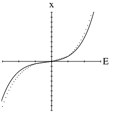
where \( T_p \) is the observed time of periapsis passage. Thus the key numerical procedure in this routine is to invert the expression \( x=E+A\sinh E+B(\cosh E - 1) \) to get \( E(x) \) . This function is sketched to the right (solid line), along with an approximation used for making an initial guess (dotted line), as described later.
We note that \( A^2-B^2<1 \) , although it approaches 1 when \( e\rightarrow1 \) , or when \( v_p\rightarrow1 \) and either \( e=0 \) or \( \omega=\pi \) . Except in this limit, Newton-Raphson methods will converge rapidly for any initial guess. In this limit, though, the slope \( dx/dE \) approaches zero at \( E=0 \) , and an initial guess or iteration landing near this point will send the next iteration off to unacceptably large or small values. A hybrid root-finding strategy is used to deal with this, and with the exponential behaviour of \( x \) at large \( E \) .
First, we compute \( x=x_{\pm1} \) at \( E=\pm1 \) . If the desired \( x \) lies in this range, we use a straightforward Newton-Raphson root finder, with the constraint that all guesses of \( E \) are restricted to the domain \( [-1,1] \) . This guarantees that the scheme will eventually find itself on a uniformly-convergent trajectory.
Second, for \( E \) outside of this range, \( x \) is dominated by the exponential terms: \( x\approx\frac{1}{2}(A+B)\exp(E) \) for \( E\gg1 \) , and \( x\approx-\frac{1}{2}(A-B)\exp(-E) \) for \( E\ll-1 \) . We therefore do an approximate Newton-Raphson iteration on the function \( \ln|x| \) , where the approximation is that we take \( d\ln|x|/d|E|\approx1 \) . This involves computing an extra logarithm inside the loop, but gives very rapid convergence to high precision, since \( \ln|x| \) is very nearly linear in these regions.
At the start of the algorithm, we use an initial guess of \( E=-\ln[-2(x-x_{-1})/(A-B)-\exp(1)] \) for \( x<x_{-1} \) , \( E=x/x_{-1} \) for \( x_{-1}\leq x\leq0 \) , \( E=x/x_{+1} \) for \( 0\leq x\leq x_{+1} \) , or \( E=\ln[2(x-x_{+1})/(A+B)-\exp(1)] \) for \( x>x_{+1} \) . We refine this guess until we get agreement to within 0.01 parts in part in \( N_\mathrm{cyc} \) (where \( N_\mathrm{cyc} \) is the larger of the number of wave cycles in a time \( 2\pi/n \) , or the number of wave cycles in the entire waveform being generated), or one part in \( 10^{15} \) (an order of magnitude off the best precision possible with REAL8 numbers). The latter case indicates that REAL8 precision may fail to give accurate phasing, and one should consider modeling the orbit as a set of Taylor frequency coefficients \'{a} la LALGenerateTaylorCW(). On subsequent timesteps, we use the previous timestep as an initial guess, which is good so long as the timesteps are much smaller than \( 1/n \) .
Once a value of \( E \) is found for a given timestep in the output series, we compute the system time \( t \) via Eq. \eqref{eq_spinorbit-t}, and use it to determine the wave phase and (non-Doppler-shifted) frequency via Eq. \eqref{eq_taylorcw-freq} and Eq. \eqref{eq_taylorcw-phi}. The Doppler shift on the frequency is then computed using Eq. \eqref{eq_spinorbit-upsilon} and Eq. \eqref{eq_orbit-rdot}. We use \( \upsilon \) as an intermediate in the Doppler shift calculations, since expressing \( \dot{R} \) directly in terms of \( E \) results in expression of the form \( (e-1)/(e\cosh E-1) \) , which are difficult to simplify and face precision losses when \( E\sim0 \) and \( e\rightarrow1 \) . By contrast, solving for \( \upsilon \) is numerically stable provided that the system atan2() function is well-designed.
This routine does not account for relativistic timing variations, and issues warnings or errors based on the criterea of Eq. \eqref{eq_relativistic-orbit} in LALGenerateEllipticSpinOrbitCW().
Definition at line 145 of file GenerateHyperbolicSpinOrbitCW.c.
| #define GENERATESPINORBITCWH_ENUL 1 |
Unexpected null pointer in arguments.
Definition at line 225 of file GenerateSpinOrbitCW.h.
| #define GENERATESPINORBITCWH_EOUT 2 |
Output field a, f, phi, or shift already exists.
Definition at line 226 of file GenerateSpinOrbitCW.h.
| #define GENERATESPINORBITCWH_EMEM 3 |
Out of memory.
Definition at line 227 of file GenerateSpinOrbitCW.h.
| #define GENERATESPINORBITCWH_EECC 4 |
Eccentricity out of range.
Definition at line 228 of file GenerateSpinOrbitCW.h.
| #define GENERATESPINORBITCWH_EFTL 5 |
Periapsis motion is faster than light.
Definition at line 229 of file GenerateSpinOrbitCW.h.
| #define GENERATESPINORBITCWH_ESGN 6 |
Sign error: positive parameter expected.
Definition at line 230 of file GenerateSpinOrbitCW.h.