Detailed Description

Provides routines to simulate generic gravitational waveforms originating from a particular source.

Author: Creighton, T. D.

Synopsis

#include <lal/PulsarSimulateCoherentGW.h>

This header covers generic routines and structures to represent and simulate the effects of a plane gravitational wave propagating from a distinct point on the sky.

Any plane gravitational wave is specified by a direction \( \mathbf{\hat{n}} \) to its apparent source (i.e. opposite to its direction of propagation), and by the inistantaneous values \( h_+(t) \) , \( h_\times(t) \) of its plus and cross polarizations as functions of (retarded) time \( t=t_0+\mathbf{\hat{n}}\cdot(\mathbf{x}-\mathbf{x}_0) \) , where \( t_0 \) is the time measured at some local reference point \( \mathbf{x}_0 \) , and \( t \) is the time measured by a synchronized clock at \( \mathbf{x} \) . We adopt the standard meaning of the instantaneous strain amplitudes \( h_{+,\times} \) : in some reference transverse \( x \) - \( y \) coordinate system oriented such that \( \mathbf{\hat{x}}\times\mathbf{\hat{y}}=-\mathbf{\hat{n}} \) points in the direction of propagation, two free observers originally separated by a displacement \( (x,y) \) will experience an additional tidal displacement \( \delta x=(xh_+ + yh_\times)/2 \) , \( \delta y=(xh_\times - yh_+)/2 \) .

Quasiperiodic waves:: Most astrophysical sources of gravitational radiation are described as quasiperiodic (or, less accurately, as "adiabatic"), in that they can be said to have an instantaneous frequency, amplitude, and polarization, all of which vary on timescales much longer than a wave period. Mathematically we write this as:
\[ h_{+,\times}(t) = A_{+,\times}(t)\cos\phi(t) + B_{+,\times}(t)\sin\phi(t) \; , \]

Polarization phase diagram for a quasiperiodic gravitational wave. The phase point p(t) traces out the indicated ellipse in the h_+\,h_x plane; the parameters A1\, A2 and Phi remain roughly constant over many cycles in phi.

where \( \phi(t)=2\pi\int f(t)\,dt \) , and the evolution timescale \( \tau=\min\{A/\dot{A},B/\dot{B},f/\dot{f}\} \) is much greater than \( h/\dot{h}\sim1/f \) . Obviously it is mathematically impossible for the physical functions \( h_{+,\times}(t) \) to specify uniquely more than two other functions of time; we rely on the notion of quasiperiodicity to define "natural" choices of instantaneous frequency and amplitude. The ambiguity in this choice is on the order of the amount that these quantities change over a cycle.

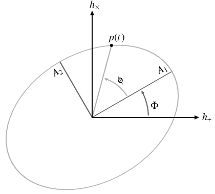
While the above formula appears to have five degrees of freedom (two quadrature amplitudes \( A \) and \( B \) for each polarization, plus a common phase function \( \phi \) ), there is a degeneracy between the two quadrature amplitudes and a shift in phase. One could simply treat each polarization independently and represent the system with two amplitude functions \( A_{+,\times} \) and two phase functions \( \phi_{+,\times} \) , but we would like to preserve the notion that the phases of the two waveforms derive from a single underlying instantaneous frequency. We therefore write the waveforms in terms of two polarization amplitudes \( A_1(t) \) and \( A_2(t) \) , a single phase function \( \phi(t) \) , and a polarization shift \( \Phi(t) \) :

\begin{eqnarray} \label{eq_quasiperiodic_hpluscross} h_+(t) & = & A_1(t)\cos\Phi(t)\cos\phi(t) - A_2(t)\sin\Phi(t)\sin\phi(t) \; , \\ h_\times(t) & = & A_1(t)\sin\Phi(t)\cos\phi(t) + A_2(t)\cos\Phi(t)\sin\phi(t) \; . \end{eqnarray}

The physical meaning of these functions is shown in this figure.

There is a close relationship between the polarization shift \( \Phi \) and the orientation of the \( x \) - \( y \) coordinates used to define our polarization basis: if we rotate the \( x \) and \( y \) axes by an angle \( \Delta\psi \) , we change \( \Phi \) by an amount \( -2\Delta\psi \) . (The factor of 2 comes from the fact that the + and \( \times \) modes are quadrupolar: a + mode rotated \( 45^\circ \) is a \( \times \) mode, and a mode rotated \( 90^\circ \) is the opposite of itself.) We use the polarization angle \( \psi \) to define the orientation of the \( x \) -axis of the polarization basis relative to an Earth-fixed reference frame (see the coordinate conventions below). If \( \Phi \) is constant, one can redefine \( \psi \) such that \( \Phi=0 \) ; however, when \( \Phi \) changes with time, we would nonetheless like our polarization basis to remain fixed. We therefore retain the constant \( \psi \) and the function \( \Phi(t) \) as distinct quantities.

The advantage of this quasiperiodic representation of a gravitational wave is that a physical sampling of the parameters \( A_1 \) , \( A_2 \) , \( \phi \) , and \( \Phi \) need only be done on timescales \( \Delta t\lesssim\tau \) , whereas the actual wave functions \( h_{+,\times} \) need to be sampled on timescales \( \Delta t\lesssim1/f \) .

The following coordinate conventions are assumed:

Fig. 7 of [35] defines standard coordinate conventions for nonprecessing binaries, and by extension, for any fixed-axis rotating source: If \( \mathbf{\hat{z}} \) points in the direction of wave propagation (away from the source), and \( \mathbf{\hat{l}} \) points in the (constant) direction of the source's angular momentum vector, then the \( x \) - \( y \) coordinates used to define the + and \( \times \) polarizations are given by \( \mathbf{\hat{x}}=|\csc i|\mathbf{\hat{z}}\times\mathbf{\hat{l}} \) and \( \mathbf{\hat{y}}=\mathbf{\hat{z}}\times\mathbf{\hat{x}} \) , where \( i=\arccos(\mathbf{\hat{z}}\cdot\mathbf{\hat{l}}) \) is the inclination angle between \( \mathbf{\hat{l}} \) and \( \mathbf{\hat{z}} \) . Such a system will generically have \( A_1(t)=A(t)(1+\cos^2i) \) , \( A_2(t)=2A(t)\cos i \) , \( \Phi(t)=0 \) , and \( f(t)>0 \) (i.e. \( \phi(t) \) increasing with time). For precessing systems, prescriptions for \( \mathbf{\hat{x}} \) and \( \mathbf{\hat{y}} \) become ambiguous, but they must be fixed; the relations for \( A_1 \) , \( A_2 \) , and \( \Phi \) will no longer be maintained.
Appendix B of [1] defines a convention for the overal polarization angle \( \psi \) : Let \( \mathbf{\hat{N}} \) be the direction of the Earth's north celestial pole, and define the direction of the ascending node \( \mathbf{\hat{\Omega}}=|\csc\alpha|\mathbf{\hat{N}}\times\mathbf{\hat{z}} \) , where \( \alpha \) is the right ascension of the source. Then \( \psi \) is the angle, right-handed about \( \mathbf{\hat{z}} \) , from \( \mathbf{\hat{\Omega}} \) to \( \mathbf{\hat{x}} \) .
The direction of propagation of the wave is defined by the right ascension \( \alpha \) and declination \( \delta \) of the source, as seen from the point of measurement. See Header SkyCoordinates.h for a definition of these quantities. We expect that these will be effectively constant for almost any gravitational wave source of interest.

The polarization response:: The relative strain induced in the test masses of a detector by a passing gravitational wave depends not only on the amplitudes \( h_{+,\times} \) of the gravitational wave, but also on the design of the detector and its orientation with relative to the \( x \) - \( y \) coordinate system used to define the + and \( \times \) polarizations. For a given detector, the response to each polarization thus depends on the right ascension \( \alpha \) , declination \( \delta \) , and polarization angle \( \psi \) of the source (which define the orientation of the + and \( \times \) polarization axes relative to the Earth), and on the time \( t \) (which determines the orientation of the detector as the Earth rotates). The strain \( h(t) \) induced in the detector is thus given by two polarization response functions \( F_{+,\times}(\alpha,\delta,\psi;t) \) by:
\[ h(t) = h_+(t)F_+(\alpha,\delta,\psi;t) + h_\times(t)F_\times(\alpha,\delta,\psi;t) \; . \]
We will not discuss the computation of these functions \( F_{+,\times} \) , as these are covered under the header Header DetResponse.h.

The transfer function:: All gravitational wave detectors incorporate a set of analog and digital filters that convert a gravitational excitation on the test masses into a measurable output time series. The effects of these functions are aggregated into a complex-valued transfer function \( {\cal T}(f) \) , which gives the instrumental response (in units of "counts" from an analog \( \rightarrow \) digital converter) to gravitational waves of unit amplitued at the frequency \( f \) . Specifically, if the strain exerted on the antenna is given by \( h(t)=\mathrm{Re}[{\cal H}e^{2\pi ift}] \) (where the complex amplitude \( \cal H \) includes the phase of the wave), then the ADC output of the instrument is given by:
\[ o(t) = \mathrm{Re}\left[ {\cal T}(f) {\cal H}e^{2\pi ift} \right] \; . \]
The transfer function has a strong frequency dependence in order to "whiten" the highly-coloured instrumental noise, and thus preserve instrumental sensitivity across a broad band of frequencies.

We note that although the transfer function measures the response of the instrument to a gravitational wave, the term response function refers to inverse transformation of taking an instrumental response and computing a gravitational waveform; that is, \( {\cal R}(f)=1/{\cal T}(f) \) . This confusing bit of nomenclature arises from the fact that most data analysis deals with extracting gravitational waveforms from the instrumental output, rather than injecting waveforms into the output.

For quasiperiodic waveforms with a well-defined instantaneous frequency \( f(t) \) and phase \( \phi(t) \) , we can compute the response of the instrument entirely in the time domain in the adiabatic limit: if our instrumental excitation is a linear superposition of waveforms \( h(t)=\mathrm{Re}[{\cal H}(t)e^{i\phi(t)}] \) , then the output is a superposition of waves of the form

\[ o(t) \approx \mathrm{Re}\left[ {\cal T}\{f(t)\} {\cal H}(t)e^{i\phi(t)} \right] \; . \]

This expression is approximate to the extent that \( {\cal T}(f) \) varies over the range \( f\pm1/\tau \) , where \( \tau \) is the evolution timescale of \( {\cal H}(t) \) and \( f(t) \) . Since the transfer function and polarization response (above) are linear operators, we can apply them in either order.

A note on terminology:: We use the word "coherent" in the name of this header in the loosest possible sense, refering to any wave with a well-defined direction of propagation, whose wave amplitudes \( h_{+,\times} \) are deterministic functions of retarded time. Given a knowledge of these parameters, such a waveform is amenable to "coherent" detection in a network of detectors, through time-shifted matched filtering.

However, coherence is often used to refer to a more restricted class of waveforms that are "effectively monochromatic" over some coherence timescale \( t_\mathrm{coh} \) ; i.e. in any timespan \( t_\mathrm{coh} \) there is a fixed-frequency sinusoid that is never more than \( 90^\circ \) out of phase with the waveform. This is more retrictive even than our concept of quasiperiodic waves; for smoothly-varying waveforms one has \( t_\mathrm{coh}\sim\dot{f}^{-1/2} \) , which is much shorter than the evolution timescale \( \tau\sim f/\dot{f} \) (provided \( \tau\gg1/f \) , as we have assumed).

Prototypes
int	XLALPulsarSimulateCoherentGW (REAL4TimeSeries output, PulsarCoherentGW CWsignal, PulsarDetectorResponse *detector)
	FIXME: Temporary XLAL-wapper to LAL-function LALPulsarSimulateCoherentGW() More...

void	LALPulsarSimulateCoherentGW (LALStatus status, REAL4TimeSeries output, PulsarCoherentGW input, PulsarDetectorResponse detector)
	Computes the response of a detector to a coherent gravitational wave. More...

Data Structures
struct	PulsarCoherentGW
	This structure stores a representation of a plane gravitational wave propagating from a particular point on the sky. More...

struct	PulsarDetectorResponse
	This structure contains information required to determine the response of a detector to a gravitational waveform. More...

Function Documentation

◆ XLALPulsarSimulateCoherentGW()

int XLALPulsarSimulateCoherentGW	(	REAL4TimeSeries *	output,
		PulsarCoherentGW *	CWsignal,
		PulsarDetectorResponse *	detector
	)

FIXME: Temporary XLAL-wapper to LAL-function LALPulsarSimulateCoherentGW()

NOTE: This violates the current version of the XLAL-spec, but is unavoidable at this time, as LALPulsarSimulateCoherentGW() hasn't been properly XLALified yet, and doing this would be beyond the scope of this patch. However, doing it here in this way is better than calling LALxxx() from various far-flung XLAL-functions, as in this way the "violation" is localized in one place, and serves as a reminder for future XLAL-ification at the same time.

Parameters

	output	[in/out] output timeseries
[in]	CWsignal	internal signal representation
[in]	detector	detector response

Definition at line 66 of file PulsarSimulateCoherentGW.c.

◆ LALPulsarSimulateCoherentGW()

void LALPulsarSimulateCoherentGW	(	LALStatus *	stat,
		REAL4TimeSeries *	output,
		PulsarCoherentGW *	CWsignal,
		PulsarDetectorResponse *	detector
	)

Computes the response of a detector to a coherent gravitational wave.

Author: Creighton, T. D.

This function takes a quasiperiodic gravitational waveform given in *signal, and estimates the corresponding response of the detector whose position, orientation, and transfer function are specified in *detector. The result is stored in *output.

The fields output->epoch, output->deltaT, and output->data must already be set, in order to specify the time period and sampling rate for which the response is required. If output->f0 is nonzero, idealized heterodyning is performed (an amount \( 2\pi f_0(t-t_0) \) is subtracted from the phase before computing the sinusoid, where \( t_0 \) is the heterodyning epoch defined in detector). For the input signal, signal->h is ignored, and the signal is treated as zero at any time for which either signal->a or signal->phi is not defined.

This routine will convert signal->position to equatorial coordinates, if necessary.

Algorithm

The routine first accounts for the time delay between the detector and the solar system barycentre, based on the detector position information stored in *detector and the propagation direction specified in *signal. Values of the propagation delay are precomuted at fixed intervals and stored in a table, with the intervals \( \Delta T_\mathrm{delay} \) chosen such that the value interpolated from adjacent table entries will never differ from the true value by more than some timing error \( \sigma_T \) . This implies that:

\[ \Delta T_\mathrm{delay} \leq \sqrt{ \frac{8\sigma_T}{\max\{a/c\}} } \; , \]

where \( \max\{a/c\}=1.32\times10^{-10}\mathrm{s}^{-1} \) is the maximum acceleration of an Earth-based detector in the barycentric frame. The total propagation delay also includes Einstein and Shapiro delay, but these are more slowly varying and thus do not constrain the table spacing. At present, a 400s table spacing is hardwired into the code, implying \( \sigma_T\approx3\mu \) s, comparable to the stated accuracy of LALBarycenter().

Next, the polarization response functions of the detector \( F_{+,\times}(\alpha,\delta) \) are computed for every 10 minutes of the signal's duration, using the position of the source in *signal, the detector information in *detector, and the function LALComputeDetAMResponseSeries(). Subsequently, the polarization functions are estimated for each output sample by interpolating these precomputed values. This guarantees that the interpolated value is accurate to \( \sim0.1\% \) .

Next, the frequency response of the detector is estimated in the quasiperiodic limit as follows:

At each sample point in *output, the propagation delay is computed and added to the sample time, and the instantaneous amplitudes \( A_1 \) , \( A_2 \) , frequency \( f \) , phase \( \phi \) , and polarization shift \( \Phi \) are found by interpolating the nearest values in signal->a, signal->f, signal->phi, and signal->shift, respectively. If signal->f is not defined at that point in time, then \( f \) is estimated by differencing the two nearest values of \( \phi \) , as \( f\approx\Delta\phi/2\pi\Delta t \) . If signal->shift is not defined, then \( \Phi \) is treated as zero.
The complex transfer function of the detector the frequency \( f \) is found by interpolating detector->transfer. The amplitude of the transfer function is multiplied with \( A_1 \) and \( A_2 \) , and the phase of the transfer function is added to \( \phi \) ,
The plus and cross contributions \( o_+ \) , \( o_\times \) to the detector output are computed as in Eq. \eqref{eq_quasiperiodic_hpluscross} of Header PulsarSimulateCoherentGW.h, but using the response-adjusted amplitudes and phase.
The final detector response \( o \) is computed as \( o=(o_+F_+)+(o_\times F_\times) \) .

A note on interpolation:

Much of the computational work in this routine involves interpolating various time series to find their values at specific output times. The algorithm is summarized below.

Let \( A_j = A( t_A + j\Delta t_A ) \) be a sampled time series, which we want to resample at new (output) time intervals \( t_k = t_0 + k\Delta t \) . We first precompute the following quantities:

\begin{eqnarray} t_\mathrm{off} & = & \frac{t_0-t_A}{\Delta t_A} \; , \\ dt & = & \frac{\Delta t}{\Delta t_A} \; . \end{eqnarray}

Then, for each output sample time \( t_k \) , we compute:

\begin{eqnarray} t & = & t_\mathrm{off} + k \times dt \; , \\ j & = & \lfloor t \rfloor \; , \\ f & = & t - j \; , \end{eqnarray}

where \( \lfloor x\rfloor \) is the "floor" function; i.e. the largest integer \( \leq x \) . The time series sampled at the new time is then:

\[ A(t_k) = f \times A_{j+1} + (1-f) \times A_j \; . \]

Notes

The major computational hit in this routine comes from computing the sine and cosine of the phase angle in Eq. \eqref{eq_quasiperiodic_hpluscross} of Header PulsarSimulateCoherentGW.h. For better online performance, these can be replaced by other (approximate) trig functions. Presently the code uses the native libm functions by default, or the function sincosp() in libsunmath if this function is available and the constant ONLINE is defined. Differences at the level of 0.01 begin to appear only for phase arguments greater than \( 10^{14} \) or so (corresponding to over 500 years between phase epoch and observation time for frequencies of around 1kHz).

To activate this feature, be sure that sunmath.h and libsunmath are on your system, and add -DONLINE to the –with-extra-cppflags configuration argument. In future this flag may be used to turn on other efficient trig algorithms on other (non-Solaris) platforms.

Definition at line 233 of file PulsarSimulateCoherentGW.c.