|
LAL 7.7.0.1-95637d2
|


|
|
LAL 7.7.0.1-95637d2
|
|

Tests the routines in Header IIRFilter.h. More...
Tests the routines in Header IIRFilter.h.
This program generates a time series vector, and passes it through a third-order Butterworth low-pass filter. By default, running this program with no arguments simply passes an impulse function to the filter routines, producing no output. All filter parameters are set from #defined constants. The following option flags are accepted:
[-f] Specifies which filter(s) to be used: filtertag is a token containing one or more character codes from a to f and/or from A to D, each corresponding to a different filter:
If not specified, -f abcd is assumed.
[-o] Prints the input and output vectors to data files: out.0 stores the initial impulse, out. c the response computed using the filter with character code c (above). If not specified, the routines are exercised, but no output is written.
[-t] Causes IIRFilterTest to fill the time series vector with Gaussian random deviates, and prints execution times for the various filter subroutines to stdout. To generate useful timing data, the default size of the time vector is increased (unless explicitly set, below).
[-d] Changes the debug level from 0 to the specified value debuglevel.
[-n] Sets the size of the time vectors to npts. If not specified, 4096 points are used (4194304 if the -t option was also given).
[-r] Applies each filter to the data reps times instead of just once.
-w] Sets the characteristic frequency of the filter to freq in the w-plane (described in ZPGFilter.h). If not specified, -w 0.01 is assumed (i.e. a characteristic frequency of 2% of Nyquist). 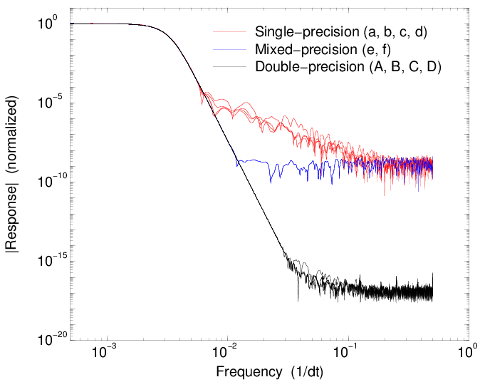
A third-order Butterworth low-pass filter is defined by the following power response function:
|T(w)|^2 = \frac{1}{1+(w/w_c)^6}\;,
where the frequency parameter w=\tan(\pi f\Delta t) maps the Nyquist interval onto the entire real axis, and w_c is the (transformed) characteristic frequency set by the -w option above. A stable time-domain filter has poles with |z|<1 in the z-plane representation, which means that the w-plane poles should have \Im(w)>0. We construct a transfer function using only the positive-imaginary poles of the power response function:
T(w) = \frac{iw_c^3}{\prod_{k=0}^2 \left[w-w_c e^{(2k+1)i\pi/6}\right]}\;,
where we have chosen a phase coefficient i in the numerator in order to get a purely real DC response. This ensures that the z-plane representation of the filter will have a real gain, resulting in a physically-realizable IIR filter.
The poles and gain of the transfer function T(w) are simply read off of the equation above, and are stored in a COMPLEX8ZPGFilter. This is transformed from the w-plane to the z-plane representation using LALWToZCOMPLEX8ZPGFilter(), and then used to create an IIR filter with LALCreateREAL4IIRFilter(). This in turn is used by the routines LALSIIRFilter(), LALIIRFilterREAL4(), LALIIRFilterREAL4Vector(), and LALIIRFilterREAL4VectorR() to filter a data vector containing either a unit impulse or white Gaussian noise (for more useful timing information).
Running this program on a 1.3 GHz Intel machine with no optimization produced the following typical timing information:
From these results it is clear that the mixed-precision vector filtering routines are the most efficient, outperforming even the purely single-precision vector filtering routines by 20%–30%. This was unanticipated; by my count the main inner loop of the single-precision routines contain 2M+2N+1 dereferences and 2M+2N-3 floating-point operations per vector element, where M and N are the direct and recursive filter orders, whereas the mixed-precision routines contain 2\max\{M,N\}+2M+2 dereferences and 2M+2N-1 floating-point operations per element. However, most of the dereferences in the mixed-precision routines are to short internal arrays rather than to the larger data vector, which might cause some speedup.
Running the same command with the -t flag replaced with -o generates files containing the impulse response of the filters. The frequency-domain impulse response is shown in this figure. This shows the steady improvement in truncation error from single- to mixed- to double-precision filtering.
Definition in file IIRFilterTest.c.
Go to the source code of this file.
Macros | |
Error Codes | |
| #define | IIRFILTERTESTC_ENORM 0 |
| Normal exit. More... | |
| #define | IIRFILTERTESTC_ESUB 1 |
| Subroutine failed. More... | |
| #define | IIRFILTERTESTC_EARG 2 |
| Error parsing arguments. More... | |
| #define | IIRFILTERTESTC_EBAD 3 |
| Bad argument value. More... | |
| #define | IIRFILTERTESTC_EFILE 4 |
| Could not create output file. More... | |
| #define IIRFILTERTESTC_ENORM 0 |
Normal exit.
Definition at line 179 of file IIRFilterTest.c.
| #define IIRFILTERTESTC_ESUB 1 |
Subroutine failed.
Definition at line 180 of file IIRFilterTest.c.
| #define IIRFILTERTESTC_EARG 2 |
Error parsing arguments.
Definition at line 181 of file IIRFilterTest.c.
| #define IIRFILTERTESTC_EBAD 3 |
Bad argument value.
Definition at line 182 of file IIRFilterTest.c.
| #define IIRFILTERTESTC_EFILE 4 |
Could not create output file.
Definition at line 183 of file IIRFilterTest.c.