Provides routines to simulate generic gravitational waveforms originating from a particular source.

Author: Creighton, T. D.

Deprecated:: This module is deprecated, please see LALSimulation for a replacement.

Synopsis

#include <lal/SimulateCoherentGW.h>

This header covers generic routines and structures to represent and simulate the effects of a plane gravitational wave propagating from a distinct point on the sky.

Any plane gravitational wave is specified by a direction \(\mathbf{\hat{n}}\) to its apparent source (i.e. opposite to its direction of propagation), and by the inistantaneous values \(h_+(t)\), \(h_\times(t)\) of its plus and cross polarizations as functions of (retarded) time \(t=t_0+\mathbf{\hat{n}}\cdot(\mathbf{x}-\mathbf{x}_0)\), where \(t_0\) is the time measured at some local reference point \(\mathbf{x}_0\), and \(t\) is the time measured by a synchronized clock at \(\mathbf{x}\). We adopt the standard meaning of the instantaneous strain amplitudes \(h_{+,\times}\): in some reference transverse \(x\)- \(y\) coordinate system oriented such that \(\mathbf{\hat{x}}\times\mathbf{\hat{y}}=-\mathbf{\hat{n}}\) points in the direction of propagation, two free observers originally separated by a displacement \((x,y)\) will experience an additional tidal displacement \(\delta x=(xh_+ + yh_\times)/2\), \(\delta y=(xh_\times - yh_+)/2\).

Quasiperiodic waves:: Most astrophysical sources of gravitational radiation are described as quasiperiodic (or, less accurately, as "adiabatic"), in that they can be said to have an instantaneous frequency, amplitude, and polarization, all of which vary on timescales much longer than a wave period. Mathematically we write this as:
\[ h_{+,\times}(t) = A_{+,\times}(t)\cos\phi(t) + B_{+,\times}(t)\sin\phi(t) \; , \]

Polarization phase diagram for a quasiperiodic gravitational wave. The phase point p(t) traces out the indicated ellipse in the h_+\,h_x plane; the parameters A1\, A2 and Phi remain roughly constant over many cycles in phi.

where \(\phi(t)=2\pi\int f(t)\,dt\), and the evolution timescale \(\tau=\min\{A/\dot{A},B/\dot{B},f/\dot{f}\}\) is much greater than \(h/\dot{h}\sim1/f\). Obviously it is mathematically impossible for the physical functions \(h_{+,\times}(t)\) to specify uniquely more than two other functions of time; we rely on the notion of quasiperiodicity to define "natural" choices of instantaneous frequency and amplitude. The ambiguity in this choice is on the order of the amount that these quantities change over a cycle.

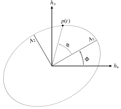
While the above formula appears to have five degrees of freedom (two quadrature amplitudes \(A\) and \(B\) for each polarization, plus a common phase function \(\phi\)), there is a degeneracy between the two quadrature amplitudes and a shift in phase. One could simply treat each polarization independently and represent the system with two amplitude functions \(A_{+,\times}\) and two phase functions \(\phi_{+,\times}\), but we would like to preserve the notion that the phases of the two waveforms derive from a single underlying instantaneous frequency. We therefore write the waveforms in terms of two polarization amplitudes \(A_1(t)\) and \(A_2(t)\), a single phase function \(\phi(t)\), and a polarization shift \(\Phi(t)\):

\begin{eqnarray} \label{eq_quasiperiodic_hpluscross} h_+(t) & = & A_1(t)\cos\Phi(t)\cos\phi(t) - A_2(t)\sin\Phi(t)\sin\phi(t) \; , \\ h_\times(t) & = & A_1(t)\sin\Phi(t)\cos\phi(t) + A_2(t)\cos\Phi(t)\sin\phi(t) \; . \end{eqnarray}

The physical meaning of these functions is shown in this figure.

There is a close relationship between the polarization shift \(\Phi\) and the orientation of the \(x\)- \(y\) coordinates used to define our polarization basis: if we rotate the \(x\) and \(y\) axes by an angle \(\Delta\psi\), we change \(\Phi\) by an amount \(-2\Delta\psi\). (The factor of 2 comes from the fact that the + and \(\times\) modes are quadrupolar: a + mode rotated \(45^\circ\) is a \(\times\) mode, and a mode rotated \(90^\circ\) is the opposite of itself.) We use the polarization angle \(\psi\) to define the orientation of the \(x\)-axis of the polarization basis relative to an Earth-fixed reference frame (see the coordinate conventions below). If \(\Phi\) is constant, one can redefine \(\psi\) such that \(\Phi=0\); however, when \(\Phi\) changes with time, we would nonetheless like our polarization basis to remain fixed. We therefore retain the constant \(\psi\) and the function \(\Phi(t)\) as distinct quantities.

The advantage of this quasiperiodic representation of a gravitational wave is that a physical sampling of the parameters \(A_1\), \(A_2\), \(\phi\), and \(\Phi\) need only be done on timescales \(\Delta t\lesssim\tau\), whereas the actual wave functions \(h_{+,\times}\) need to be sampled on timescales \(\Delta t\lesssim1/f\).

The following coordinate conventions are assumed:

Fig. 7 of [29] defines standard coordinate conventions for nonprecessing binaries, and by extension, for any fixed-axis rotating source: If \(\mathbf{\hat{z}}\) points in the direction of wave propagation (away from the source), and \(\mathbf{\hat{l}}\) points in the (constant) direction of the source's angular momentum vector, then the \(x\)- \(y\) coordinates used to define the + and \(\times\) polarizations are given by \(\mathbf{\hat{x}}=|\csc i|\mathbf{\hat{z}}\times\mathbf{\hat{l}}\) and \(\mathbf{\hat{y}}=\mathbf{\hat{z}}\times\mathbf{\hat{x}}\), where \(i=\arccos(\mathbf{\hat{z}}\cdot\mathbf{\hat{l}})\) is the inclination angle between \(\mathbf{\hat{l}}\) and \(\mathbf{\hat{z}}\). Such a system will generically have \(A_1(t)=A(t)(1+\cos^2i)\), \(A_2(t)=2A(t)\cos i\), \(\Phi(t)=0\), and \(f(t)>0\) (i.e. \(\phi(t)\) increasing with time). For precessing systems, prescriptions for \(\mathbf{\hat{x}}\) and \(\mathbf{\hat{y}}\) become ambiguous, but they must be fixed; the relations for \(A_1\), \(A_2\), and \(\Phi\) will no longer be maintained.
Appendix B of [4] defines a convention for the overal polarization angle \(\psi\): Let \(\mathbf{\hat{N}}\) be the direction of the Earth's north celestial pole, and define the direction of the ascending node \(\mathbf{\hat{\Omega}}=|\csc\alpha|\mathbf{\hat{N}}\times\mathbf{\hat{z}}\), where \(\alpha\) is the right ascension of the source. Then \(\psi\) is the angle, right-handed about \(\mathbf{\hat{z}}\), from \(\mathbf{\hat{\Omega}}\) to \(\mathbf{\hat{x}}\).
The direction of propagation of the wave is defined by the right ascension \(\alpha\) and declination \(\delta\) of the source, as seen from the point of measurement. See Header SkyCoordinates.h for a definition of these quantities. We expect that these will be effectively constant for almost any gravitational wave source of interest.

The polarization response:: The relative strain induced in the test masses of a detector by a passing gravitational wave depends not only on the amplitudes \(h_{+,\times}\) of the gravitational wave, but also on the design of the detector and its orientation with relative to the \(x\)- \(y\) coordinate system used to define the + and \(\times\) polarizations. For a given detector, the response to each polarization thus depends on the right ascension \(\alpha\), declination \(\delta\), and polarization angle \(\psi\) of the source (which define the orientation of the + and \(\times\) polarization axes relative to the Earth), and on the time \(t\) (which determines the orientation of the detector as the Earth rotates). The strain \(h(t)\) induced in the detector is thus given by two polarization response functions \(F_{+,\times}(\alpha,\delta,\psi;t)\) by:
\[ h(t) = h_+(t)F_+(\alpha,\delta,\psi;t) + h_\times(t)F_\times(\alpha,\delta,\psi;t) \; . \]
We will not discuss the computation of these functions \(F_{+,\times}\), as these are covered under the header Header DetResponse.h.

The transfer function:: All gravitational wave detectors incorporate a set of analog and digital filters that convert a gravitational excitation on the test masses into a measurable output time series. The effects of these functions are aggregated into a complex-valued transfer function \({\cal T}(f)\), which gives the instrumental response (in units of "counts" from an analog \(\rightarrow\)digital converter) to gravitational waves of unit amplitued at the frequency \(f\). Specifically, if the strain exerted on the antenna is given by \(h(t)=\mathrm{Re}[{\cal H}e^{2\pi ift}]\) (where the complex amplitude \(\cal H\) includes the phase of the wave), then the ADC output of the instrument is given by:
\[ o(t) = \mathrm{Re}\left[ {\cal T}(f) {\cal H}e^{2\pi ift} \right] \; . \]
The transfer function has a strong frequency dependence in order to "whiten" the highly-coloured instrumental noise, and thus preserve instrumental sensitivity across a broad band of frequencies.

We note that although the transfer function measures the response of the instrument to a gravitational wave, the term response function refers to inverse transformation of taking an instrumental response and computing a gravitational waveform; that is, \({\cal R}(f)=1/{\cal T}(f)\). This confusing bit of nomenclature arises from the fact that most data analysis deals with extracting gravitational waveforms from the instrumental output, rather than injecting waveforms into the output.

For quasiperiodic waveforms with a well-defined instantaneous frequency \(f(t)\) and phase \(\phi(t)\), we can compute the response of the instrument entirely in the time domain in the adiabatic limit: if our instrumental excitation is a linear superposition of waveforms \(h(t)=\mathrm{Re}[{\cal H}(t)e^{i\phi(t)}]\), then the output is a superposition of waves of the form

\[ o(t) \approx \mathrm{Re}\left[ {\cal T}\{f(t)\} {\cal H}(t)e^{i\phi(t)} \right] \; . \]

This expression is approximate to the extent that \({\cal T}(f)\) varies over the range \(f\pm1/\tau\), where \(\tau\) is the evolution timescale of \({\cal H}(t)\) and \(f(t)\). Since the transfer function and polarization response (above) are linear operators, we can apply them in either order.

A note on terminology:: We use the word "coherent" in the name of this header in the loosest possible sense, refering to any wave with a well-defined direction of propagation, whose wave amplitudes \(h_{+,\times}\) are deterministic functions of retarded time. Given a knowledge of these parameters, such a waveform is amenable to "coherent" detection in a network of detectors, through time-shifted matched filtering.

However, coherence is often used to refer to a more restricted class of waveforms that are "effectively monochromatic" over some coherence timescale \(t_\mathrm{coh}\); i.e. in any timespan \(t_\mathrm{coh}\) there is a fixed-frequency sinusoid that is never more than \(90^\circ\) out of phase with the waveform. This is more retrictive even than our concept of quasiperiodic waves; for smoothly-varying waveforms one has \(t_\mathrm{coh}\sim\dot{f}^{-1/2}\), which is much shorter than the evolution timescale \(\tau\sim f/\dot{f}\) (provided \(\tau\gg1/f\), as we have assumed).