Module TerrestrialCoordinates.c

Detailed Description

Converts among equatorial, geographic, and horizon coordinates.

Author

Creighton, T. D.

The functions LALEquatorialToGeographic() and LALGeographicToEquatorial() convert between equatorial and geographic coordinate systems, reading coordinates in the first system from *input and storing the new coordinates in *output. The two pointers may point to the same object, in which case the conversion is done in place. The functions will also check input->system and set output->system as appropriate. Because the geographic coordinate system is not fixed, one must also specify the time of the transformation in *gpsTime.

The function LALSystemToHorizon() transforms coordinates from either celestial equatorial coordinates or geographic coordinates to a horizon coordinate system, reading coordinates in the first system from *input and storing the horizon coordinates in *output, as above. The parameter *zenith specifies the direction of the vertical axis in the original coordinate system; the routine checks to see that input->system and zenith->system agree. Normally this routine is used to convert from geographic latitude and longitude to a horizon system, in which case *zenith simply stores the geographic (geodetic) coordinates of the observer; if converting from equatorial coordinates, zenith->longitude should store the local mean sidereal time of the horizon system.

The function LALHorizonToSystem() does the reverse of the above, transforming coordinates from horizon coordinates to either equatorial or geographic coordinates as specified by zenith->system; the value of output->system is set to agree with zenith->system.

Although it is conventional to specify an observation location by its geodetic coordinates, some routines may provide or require geocentric coordinates. The routines LALGeocentricToGeodetic() and LALGeodeticToGeocentric() perform this computation, reading and writing to the variable parameter structure *location. The function LALGeocentricToGeodetic() reads the fields location->x, y, z, and computes location->zenith and location->altitude. The function LALGeodeticToGeocentric() does the reverse, and also sets the fields location->position and location->radius.

Algorithm

These routines follow the formulae in Sec. 5.1 of [15] , which we reproduce below.

Geographic coordinates:

Since geographic and equatorial coordinates share the same \(z\)-axis, the geographic latitude \(\phi\) of a direction in space is the same as its declination \(\delta\), and longitude \(\lambda\) and right ascension \(\alpha\) differ only through the rotation of the Earth:

\begin{equation} \label{eq_lambda_geographic} \lambda = \alpha - \left(\frac{2\pi\,\mathrm{radians}} {24\,\mathrm{hours}}\right)\times\mathrm{GMST} \; , \end{equation}

where GMST is Greenwich mean sidereal time. The conversion routines here simply use the functions in the date package to compute GMST for a given GPS time, and add it to the longitude. While this is simple enough, it does involve several function calls, so it is convenient to collect these into one routine.

Horizon coordinates:

We correct a typographical error on the second line of Eq. 5.45 of [15] , (it should have \(\cos A\), not \(\sin A\)). We also note that while our latitudinal coordinate is just the altitude \(a\) in this system, our longitudinal coordinate increases counterclockwise, and thus corresponds to the negative of the azimuth \(A\) as defined by [15] . So we have:

\begin{eqnarray} \label{eq_altitude_horizon} a & = & \arcsin(\sin\delta\sin\phi + \cos\delta\cos\phi\cos h) \; , \\ \label{eq_azimuth_horizon} -A & = & \arctan\!2(\cos\delta\sin h, \sin\delta\cos\phi - \cos\delta\sin\phi\cos h) \; , \end{eqnarray}

where \(\delta\) is the declination (geographic latitude) of the direction being transformed, \(\phi\) is the geographic latitude of the observer's zenith (i.e. the observer's geodetic latitude), and \(h\) is the hour angle of the direction being transformed. This is defined as:

\begin{eqnarray} h & = & \lambda_\mathrm{zenith} - \lambda\\ & = & \mathrm{LMST} - \alpha \end{eqnarray}

where LMST is the local mean sidereal time at the point of observation. The inverse transformation is:

\begin{eqnarray} \label{eq_delta_horizon} \delta & = & \arcsin(\sin a\sin\phi + \cos a\cos A\cos\phi) \; , \\ \label{eq_h_horizon} h & = & \arctan\!2[\cos a\sin(-A), \sin a\cos\phi - \cos a\cos A\sin\phi] \; . \end{eqnarray}

As explained in Module CelestialCoordinates.c, the function \(\arctan\!2(y,x)\) returns the argument of the complex number \(x+iy\).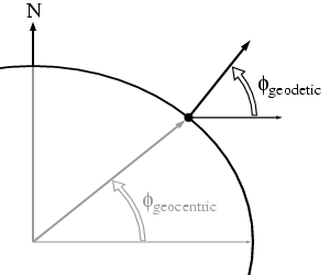

The difference between geodetic and geocentric latitude.

Geocentric coordinates:

As shown in this figure, the ellipticity of the Earth means that the vertical axis of a point on the Earth's surface does not pass through the geometric centre of the Earth. This means that the geodetic latitude of a location (defined as the latitude angle \(\phi_\mathrm{geodetic}\) of that location's zenith direction) is typically some 10 arcminutes larger than its geocentric latitude (defined as the latitude angle \(\phi_\mathrm{geographic}\) of the position vector from the geocentre through the location). Cartographers traditionally refer to locations by their geodetic coordinates, since these can be determined locally; however, geocentric coordinates are required if one wants to construct a uniform Cartesian system for the Earth as a whole.

To transform from geodetic to geocentric coordinates, one first defines a "reference ellipsoid", the best-fit ellipsoid to the surface of the Earth. This is specified by the polar and equatorial radii of the Earth \(r_p\) and \(r_e\), or equivalently by \(r_e\) and a flattening factor:

\[ f \equiv 1 - \frac{r_p}{r_e} = 0.00335281 \; . \]

(This constant will eventually migrate into Header LALConstants.h.) The surface of the ellipsoid is then specified by the equation

\[ r = r_e ( 1 - f\sin^2\phi ) \; , \]

where \(\phi=\phi_\mathrm{geodetic}\) is the geodetic latitude. For points off of the reference ellipsoid, the transformation from geodetic coordinates \(\lambda\), \(\phi\) to geocentric Cartesian coordinates is:

\begin{eqnarray} x & = & ( r_e C + h ) \cos\phi\cos\lambda \; , \\ y & = & ( r_e C + h ) \cos\phi\sin\lambda \; , \\ z & = & ( r_e S + h ) \sin\phi \; , \end{eqnarray}

where

\begin{eqnarray} C & = & \frac{1}{\sqrt{\cos^2\phi + (1-f)^2\sin^2\phi}} \; , \\ S & = & (1-f)^2 C \; , \end{eqnarray}

and \(h\) is the perpendicular elevation of the location above the reference ellipsoid. The geocentric spherical coordinates are given simply by:

\begin{eqnarray} r & = & \sqrt{ x^2 + y^2 + z^2 } \; , \\ \lambda_\mathrm{geocentric} & = & \lambda \quad = \quad \lambda_\mathrm{geodetic} \; , \\ \phi_\mathrm{geocentric} & = & \arcsin( z/r ) \; . \end{eqnarray}

When computing \(r\) we are careful to factor out the largest component before computing the sum of squares, to avoid floating-point overflow; however this should be unnecessary for radii near the surface of the Earth.

The inverse transformation is somewhat trickier. Eq. 5.29 of [15] conveniently gives the transformation in terms of a sequence of intermediate variables, but unfortunately these variables are not particularly computer-friendly, in that they are prone to underflow or overflow errors. The following equations essentially reproduce this sequence using better-behaved methods of calculation.

Given geocentric Cartesian coordinates \(x=r\cos\phi_\mathrm{geocentric}\cos\lambda\), \(y=r\cos\phi_\mathrm{geocentric}\sin\lambda\), and \(z=r\sin\phi_\mathrm{geocentric}\), one computes the following:

\begin{eqnarray} \varpi & = & \sqrt{ \left(\frac{x}{r_e}\right)^2 + \left(\frac{y}{r_e}\right)^2 } \;,\\ E & = & (1-f)\left|\frac{z}{r_e}\right| - f(2-f) \;,\\ F & = & (1-f)\left|\frac{z}{r_e}\right| + f(2-f) \;,\\ P & = & \frac{4}{3}\left( EF + \varpi^2 \right) \quad = \quad \frac{4}{3}\left[ \varpi^2 + (1-f)^2\left(\frac{z}{r_e}\right)^2 - f^2(2-f)^2 \right] \;,\\ Q & = & 2\varpi(F^2 - E^2) \quad = \quad 8\varpi f(1-f)(2-f)\left|\frac{z}{r_e}\right| \;,\\ D & = & P^3 + Q^2 \;,\\ v & = & \left\{\begin{array}{lr} \left(\sqrt{D}+Q\right)^{1/3} - \left(\sqrt{D}-Q\right)^{1/3} & D\geq0 \\ 2\sqrt{-P}\cos\left(\frac{1}{3} \arccos\left[\frac{Q}{-P\sqrt{-P}}\right]\right) & D\leq0 \end{array}\right.\\ W & = & \sqrt{E^2 + \varpi v}\\ G & = & \frac{1}{2}\left(E+W\right)\;,\\ t & = & \sqrt{G^2+\frac{\varpi^2 F - \varpi vG}{W}}-G \;. \end{eqnarray}

Once we have \(t\) and \(\varpi\), we can compute the geodetic longitude \(\lambda\), latitude \(\phi\), and elevation \(h\):

\begin{eqnarray} \lambda & = & \arctan\!2(y,x) \; , \\ \phi & = & \mathrm{sgn}({z})\arctan\left[\frac{1}{2(1-f)} \left(\frac{(\varpi-t)(\varpi+t)}{\varpi t}\right)\right] \; , \\ h & = & r_e(\varpi-t/\varpi)\cos\phi + [z-\mathrm{sgn}({z})r_e(1-f)]\sin\phi \; . \end{eqnarray}

Singular surfaces in the geodetic coordinate system. The ellipticity of this spheroid has been exaggerated compared with the Earth.

These formulae still leave certain areas where coordinate singularities or numerical cancelations can occur. Some of these have been dealt with in the code:

• There is a coordinate singularity at \(\varpi=0\), which we deal with by setting \(\phi=\pm90^\circ\) and \(\lambda\) arbitrarily to \(0^\circ\). When \(z=0\) as well, we arbitrarily choose the positive sign for \(\phi\). As \(\varpi\rightarrow0\), there are cancellations in the computation of \(G\) and \(t\), which call for special treatment (below).

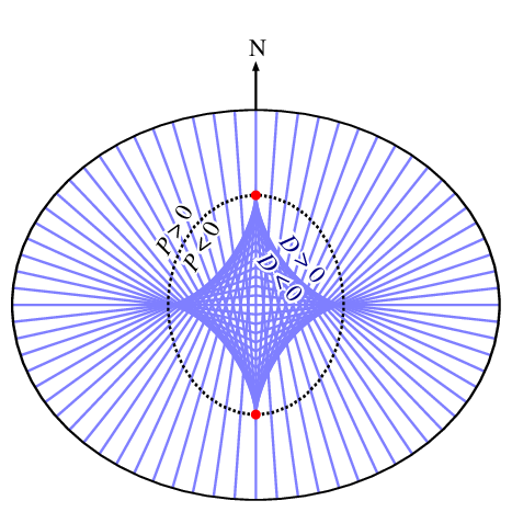
• There is another coordinate singularity when \(D\leq0\), where lines of constant geodetic latitude will cross each other, as shown in this figure. That is, a given point within this region can be assigned a range of geodetic latitudes. The multi-valued region lies within an inner ellipsoid \(P\leq0\), which in the case of the Earth has equatorial radius \(r_0=r_ef(2-f)=42.6977\)km and axial height \(z_0=r_0/(1-f)=42.8413\)km. The formula for \(v\), above, has an analytic continuation to \(D\leq0\), assigning consistent (though not unique) values of latitute and elevation to these points.

• Near the equator we have \(Q\rightarrow0\), and the first expression for \(v\) becomes a difference of nearly-equal numbers, leading to loss of precision. To deal with this, we write that expression for \(v\) as:

  \[ \begin{array}{rcl@{\qquad}c@{\qquad}l} v &=& D^{1/6}\left[(1+B)^{1/3}-(1-B)^{1/3}\right] &\mbox{where}& B \;\;=\;\; \displaystyle \frac{Q}{\sqrt{D}} \\ &\approx& D^{1/6}\left[\frac{2}{3}B+\frac{10}{81}B^3\right] &\mbox{as}& B \;\;\rightarrow\;\;0 \end{array} \]

  The switch from the "exact" formula to the series expansion is done for \(B<10^{-3}\) (within about \(2^\circ\) of the equator). This was found by experimentation to be the point where the inaccuracy of the series expansion is roughly equal to the imprecision in evaluating the "exact" formula. The resulting position errors are of order 1 part in \(10^{12}\) or less; i.e. about 3–4 digits loss of precision.

• In some places we have expressions of the form \(\sqrt{a^2+b}-a\), which becomes a difference of nearly equal numbers for \(|b|\ll a^2\), resulting in loss of precision. There are three distinct lines or surfaces where this occurs:

  1. Near the ellipsoidal surface \(P\approx0\), the expression \(\sqrt{D}-Q\) in the equation for \(v\) becomes of this form.
  2. Near the polar axis \(\varpi\approx0\), the expression for \(t\) becomes of this form.
  3. Near the polar axis \(\varpi\approx0\) within the inner ellipsoid, we have \(E<0\) and the expression for \(G\) becomes of this form.

  In each case, we expand in the small parameter \(H=b/a^2\), giving:

  \[ \sqrt{a^2+b}-a \;\;\approx\;\; a\left(\frac{1}{2} H - \frac{1}{8} H^2 + \frac{1}{16} H^3\right) \qquad\mbox{for}\qquad |H| = \left|\frac{b}{a^2}\right| \ll 1 \]

  We switch to the series expansion for \(|H|<\times10^{-4}\), which again is the point where residual errors in the series expansion are about the same as the loss of precision without the expansion. This formula converges much better than the one for \(v\) (above), resulting in negligible loss of precision in the final position.

• The only remaining known numerical singularities are at the poles of the inner ellipsoid, shown as red dots in this figure. These points stubbornly resist high-precision calculation. However, they are extremely unlikely to come up in practice.

Ellipsoidal vs. orthometric elevation:

In this module it is assumed that all elevations refer heights above the reference ellipsoid. This is the elevation computed by such techniques as GPS triangulation. However, the "true" orthometric elevation refers to the height above the mean sea level or geoid, a level surface in the Earth's gravitational potential. Thus, even if two points have the same ellipsoidal elevation, water will still flow from the higher to the lower orthometric elevation.

The difference between the geoid and reference ellipsoid is called the "undulation of the geoid", and can vary by over a hundred metres over the Earth's surface. However, it can only be determined through painstaking measurements of local variations in the Earth's gravitational field. For this reason we will ignore the undulation of the geoid.

Uses

XLALGreenwichMeanSiderealTime()

Prototypes
void	LALEquatorialToGeographic (LALStatus *stat, SkyPosition *output, SkyPosition *input, LIGOTimeGPS *gpsTime)
void	LALGeographicToEquatorial (LALStatus *stat, SkyPosition *output, SkyPosition *input, LIGOTimeGPS *gpsTime)
void	LALSystemToHorizon (LALStatus *stat, SkyPosition *output, SkyPosition *input, const SkyPosition *zenith)
void	LALHorizonToSystem (LALStatus *stat, SkyPosition *output, SkyPosition *input, const SkyPosition *zenith)
void	LALGeodeticToGeocentric (LALStatus *stat, EarthPosition *location)
void	LALGeocentricToGeodetic (LALStatus *stat, EarthPosition *location)

Function Documentation

LALEquatorialToGeographic()

void LALEquatorialToGeographic	(	LALStatus *	stat,
		SkyPosition *	output,
		SkyPosition *	input,
		LIGOTimeGPS *	gpsTime
	)

See also

See documentation in Module TerrestrialCoordinates.c

Definition at line 345 of file TerrestrialCoordinates.c.

LALGeographicToEquatorial()

void LALGeographicToEquatorial	(	LALStatus *	stat,
		SkyPosition *	output,
		SkyPosition *	input,
		LIGOTimeGPS *	gpsTime
	)

See also

See documentation in Module TerrestrialCoordinates.c

Definition at line 379 of file TerrestrialCoordinates.c.

LALSystemToHorizon()

void LALSystemToHorizon	(	LALStatus *	stat,
		SkyPosition *	output,
		SkyPosition *	input,
		const SkyPosition *	zenith
	)

See also

See documentation in Module TerrestrialCoordinates.c

Definition at line 413 of file TerrestrialCoordinates.c.

LALHorizonToSystem()

void LALHorizonToSystem	(	LALStatus *	stat,
		SkyPosition *	output,
		SkyPosition *	input,
		const SkyPosition *	zenith
	)

See also

See documentation in Module TerrestrialCoordinates.c

Definition at line 468 of file TerrestrialCoordinates.c.

LALGeodeticToGeocentric()

void LALGeodeticToGeocentric	(	LALStatus *	stat,
		EarthPosition *	location
	)

See also

See documentation in Module TerrestrialCoordinates.c

Definition at line 522 of file TerrestrialCoordinates.c.

LALGeocentricToGeodetic()

void LALGeocentricToGeodetic	(	LALStatus *	stat,
		EarthPosition *	location
	)

See also

See documentation in Module TerrestrialCoordinates.c

Definition at line 577 of file TerrestrialCoordinates.c.