Bounded KDEs
In many situations, we may have a set of samples which are bounded by a given domain. For this case, the standard scipy.stats.gaussian_kde will not accurately capture the true shape of the distribution. For cases like this, we require a bounded KDE.
There are a number of ways to take into account the bounded nature of the distribution. The common methods include: - Reflective: Making the boundaries reflective, i.e. the derivative is zero at the boundary. - Transform: Where the values are transformed to new coordinates in which the PDF does not have a boundary and looks close to Gaussian. This makes it easier for scipy.stats.gaussian_kde to represent the distribution. - Periodic: Where the values are translated into new coordinates in which the PDF does not have a boundary. This makes it easier for scipy.stats.gaussian_kde to represent the distribution.
pesummary handles bounded KDEs through the pesummary.core.plots.bounded_1d_kde module. Below is an example which shows a distribution which is bounded in the domain 0 < x < 1. We show how each method handles the boundary:
>>> from pesummary.core.plots.bounded_1d_kde import bounded_1d_kde
>>> import numpy as np
>>> from scipy import stats
>>> import matplotlib.pyplot as plt
>>> rands = np.random.random_sample(10000)
>>> transf = 0.5 + np.arcsin(2. * rands - 1.) / np.pi
>>> fig = plt.figure()
>>> plt.hist(transf, bins=50, density=True, histtype="step")
>>> xsmooth = np.linspace(0., 1., 100)
>>> unbounded_kde = stats.gaussian_kde(transf)
>>> reflection = bounded_1d_kde(transf, xlow=0., xhigh=1., method="Reflection")
>>> transform = bounded_1d_kde(transf, xlow=0., xhigh=1., method="Transform", smooth=2)
>>> periodic = bounded_1d_kde(transf, xlow=0., xhigh=1., method="Periodic")
>>> plt.plot(xsmooth, unbounded_kde(xsmooth), label="gaussiankde")
>>> plt.plot(xsmooth, reflection(xsmooth), label="reflection")
>>> plt.plot(xsmooth, transform(xsmooth), label="transform")
>>> plt.plot(xsmooth, periodic(xsmooth), label="periodic")
>>> plt.ylabel("Probability Density")
>>> plt.legend()
>>> plt.show()

Of course, different techniques for handling the boundaries are useful in different situations. Clearly, the transform method is best for the example above. Below we show an example where the reflection method is best:
>>> xsmooth = np.linspace(0., 1., 100)
>>> pts = np.random.uniform(0, 1, 10000)
>>> fig = plt.figure()
>>> plt.hist(pts, bins=50, density=True, histtype="step")
>>> unbounded_kde = stats.gaussian_kde(pts)
>>> reflection = bounded_1d_kde(pts, xlow=0., xhigh=1., method="Reflection")
>>> transform = bounded_1d_kde(pts, xlow=0., xhigh=1., method="Transform", smooth=6)
>>> periodic = bounded_1d_kde(pts, xlow=0., xhigh=1., method="Periodic")
>>> plt.plot(xsmooth, unbounded_kde(xsmooth), label="gaussiankde")
>>> plt.plot(xsmooth, reflection(xsmooth), label="reflection")
>>> plt.plot(xsmooth, transform(xsmooth), label="transform")
>>> plt.plot(xsmooth, periodic(xsmooth), label="periodic")
>>> plt.ylabel("Probability Density")
>>> plt.legend()
>>> plt.show()

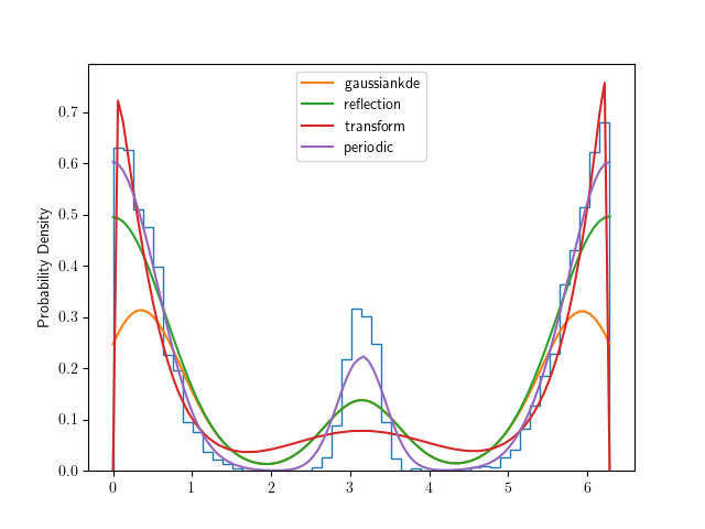
And finally an example where the periodic method is best:
>>> xsmooth = np.linspace(0., 2*np.pi, 100)
>>> pts = np.random.normal(0, 0.5, 5000)
>>> pts[pts < 0] += 2*np.pi
>>> pts = np.append(pts, np.random.normal(np.pi, 0.2, 1000))
>>> fig = plt.figure()
>>> plt.hist(pts, bins=50, density=True, histtype="step")
>>> unbounded_kde = stats.gaussian_kde(pts)
>>> reflection = bounded_1d_kde(pts, xlow=0., xhigh=2*np.pi, method="Reflection")
>>> transform = bounded_1d_kde(pts, xlow=0., xhigh=2*np.pi, method="Transform", smooth=6)
>>> periodic = bounded_1d_kde(pts, xlow=0., xhigh=2*np.pi, method="Periodic", smooth=1)
>>> plt.plot(xsmooth, unbounded_kde(xsmooth), label="gaussiankde")
>>> plt.plot(xsmooth, reflection(xsmooth), label="reflection")
>>> plt.plot(xsmooth, transform(xsmooth), label="transform")
>>> plt.plot(xsmooth, periodic(xsmooth), label="periodic")
>>> plt.ylabel("Probability Density")
>>> plt.legend()
>>> plt.show()