Plotting gravitational wave strain data
When LIGO/Virgo announces a gravitational wave, both the samples and gravitational wave data are released to the public. Through pesummary’s pesummary.gw.file.strain module, we can not only plot the gravitational wave data, but we can also compare it to the maximum likelihood waveform from the parameter estimation analysis. Below we show an example for GW150914,
 1from pesummary.gw.file.strain import StrainData
 2from pesummary.io import read
 3import subprocess
 4
 5# First we download the GW150914 posterior samples. We use the posterior
 6# samples generated by the `bilby` python package
 7subprocess.check_call(
 8    "curl https://dcc.ligo.org/public/0168/P2000193/002/pesummary_samples.zip -o pesummary_samples.zip", shell=True
 9)
10subprocess.check_call("unzip pesummary_samples.zip", shell=True)
11
12# Next we fetch the LIGO Livingston data around the time of GW150914
13L1_data = StrainData.fetch_open_data('L1', 1126259446, 1126259478)
14
15# We then read in the posterior samples and generate the maximum likelihood
16# waveform in the time domain
17samples = read("pesummary_samples/GW150914_bilby_pesummary.dat").samples_dict
18maxL = samples.maxL_td_waveform("IMRPhenomPv2", 1. / 2048, 20., project="L1")
19
20# Next we plot the data
21fig = L1_data.plot(
22    type="td", merger_time=1126259462.4, window=(-0.1, 0.1),
23    template={"L1": maxL}, bandpass_frequencies=[40., 300.]
24)
25fig.savefig("GW150914.png")
26fig.close()

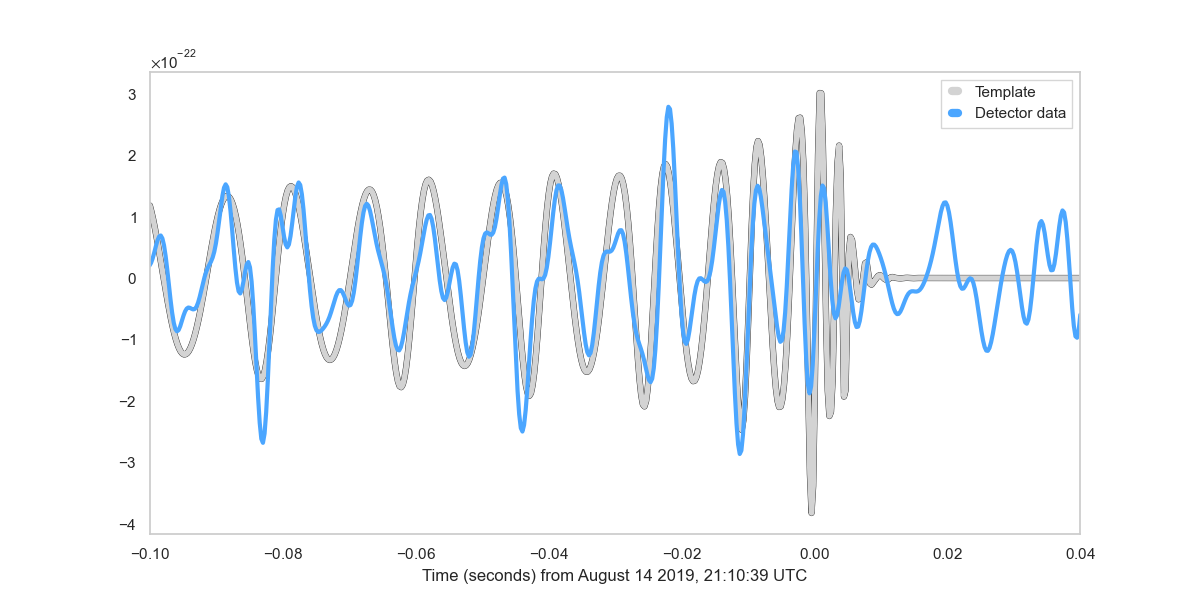
and GW190814,
 1from pesummary.gw.file.strain import StrainData
 2from pesummary.gw.fetch import fetch_open_samples
 3
 4# First we download the GW190814 posterior samples and generate the maximum
 5# likelihood waveform in the time domain
 6data = fetch_open_samples("GW190814", unpack=True, path="GW190814.h5")
 7samples = data.samples_dict["C01:SEOBNRv4PHM"]
 8maxL = samples.maxL_td_waveform("SEOBNRv4PHM", 1. / 4096, 20., project="L1")
 9
10# # Next we fetch the LIGO Livingston data around the time of GW190814
11L1_data = StrainData.fetch_open_data('L1', 1249852257.01 - 20, 1249852257.01 + 5)
12
13# Next we plot the data
14fig = L1_data.plot(
15    type="td", merger_time=1249852257.01, window=(-0.1, 0.04),
16    template={"L1": maxL}, bandpass_frequencies=[50., 300.]
17)
18fig.savefig("GW190814.png")
19fig.close()