Remaking plots that appear in GWTC1
Here we will go through step by step how to make all plots that appear in the GWTC1 paper produced by the LIGO Virgo collaboration. This involves first downloading the data, and then using the summarypublication executable provided by PESummary.
 1# Here I will show you how to recreate the plots in GWTC1 using the
 2# summarypublication executable. Note that we cannot reproduce all of the
 3# plots in GWTC1 because the data release does not hold all of the required
 4# parameters
 5
 6# First, we need to download the data from the DCC
 7curl -O https://dcc.ligo.org/public/0157/P1800370/004/GWTC-1_sample_release.tar.gz
 8tar -xf GWTC-1_sample_release.tar.gz
 9
10# Lets remove the priorChoice files as they do not contain posterior samples
11FILES_TO_REMOVE=($(ls ./GWTC-1_sample_release/*priorChoices*))
12for i in ${FILES_TO_REMOVE[@]}; do
13    rm ${i}
14done
15
16# Now lets get a list of all of the files
17FILES=($(ls ./GWTC-1_sample_release/*_GWTC-1.hdf5))
18
19# Now lets get a list of labels
20LABELS=()
21for i in ${FILES[@]}; do
22    label=`python -c "print('${i}'.split('_GWTC-1.hdf5')[0])"`
23    LABELS+=(`python -c "print('${label}'.split('./GWTC-1_sample_release/')[1])"`)
24done
25
26# Now lets assign the same colors and linestyles that were used in GWTC1
27COLORS=('#00a7f0' '#9da500' '#c59700' '#55b300' '#f77b00' '#ea65ff' '#00b1a4' '#00b47d' '#ff6c91' '#00aec2' '#9f8eff')
28LINESTYLES=(solid dashed solid solid dashed solid solid dashed solid dashed dashed)
Now that we have all of the data and all of the variables setup, we can now run the summarypublication executable and make a 2d bounded contour of the mass_1 and mass_2 parameter space
1summarypublication --plot 2d_contour \
2                   --webdir ./GWTC-1_sample_release \
3                   --samples ${FILES[@]} \
4                   --labels ${LABELS[@]} \
5                   --parameters mass_1 mass_2 \
6                   --colors ${COLORS[@]} \
7                   --linestyles ${LINESTYLES[@]} \

Now we can produced a violin plot showing the variation in mass_ratio
1# Top left panel of figure 5
2summarypublication --plot violin \
3                   --webdir ./GWTC-1_sample_release \
4                   --samples ${FILES[@]} \
5                   --labels ${LABELS[@]} \
6                   --parameters mass_ratio \

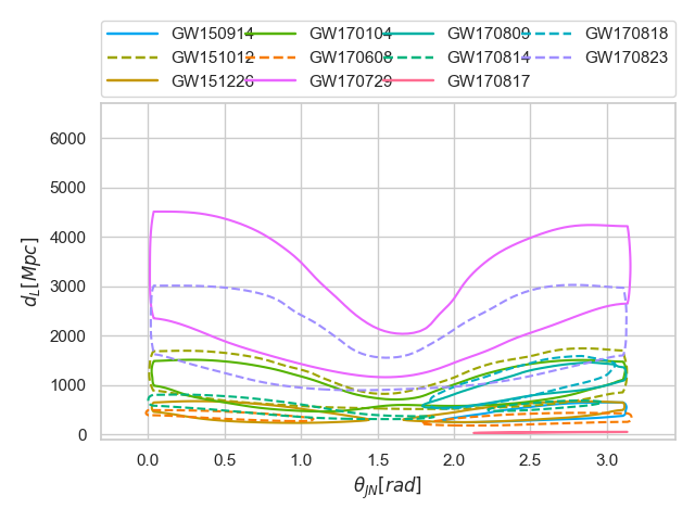
Now we can produce a 2d bounded contour of the theta_jn and luminosity_distance parameter space
1# Left panel of Figure 7
2summarypublication --plot 2d_contour \
3                   --webdir ./GWTC-1_sample_release \
4                   --samples ${FILES[@]} \
5                   --labels ${LABELS[@]} \
6                   --parameters theta_jn luminosity_distance \
7                   --colors ${COLORS[@]} \
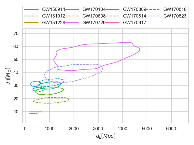
Now we can produce a 2d bounded contour of the luminosity_distance chirp_mass parameter space
1# Right panel of Figure 8
2summarypublication --plot 2d_contour \
3                   --webdir ./GWTC-1_sample_release \
4                   --samples ${FILES[@]} \
5                   --labels ${LABELS[@]} \
6                   --parameters luminosity_distance chirp_mass \
7                   --colors ${COLORS[@]} \