Comparing posterior samples from different groups
As a result of the public release of the gravitational wave strain data, groups
outside of LIGO–Virgo have also been able to analyse the gravitational wave
strain data and obtain posterior samples for a series of events. For example,
see the
2-OGC: Open Gravitational-wave Catalog of binary mergers from analysis of public Advanced LIGO and Virgo data
and
New binary black hole mergers in the second observing run of Advanced LIGO and Advanced Virgo
papers. Below, we show that pesummary provides an easy method for
comparing the posterior samples obtained by these different groups.
1from pesummary.utils.samples_dict import MultiAnalysisSamplesDict
2
3# Define a dictionary of kwargs which are used to load the result files. These
4# kwargs are passed directly to the `pesummary.io.read` function.
5load_kwargs = {
6 "princeton": dict(file_format="princeton"),
7 "pycbc": dict(path_to_samples="samples")
8}
9
10# Load the data into a MultiAnalysisSamplesDict class using the `.from_files`
11# class method. Here we are passing URLs. PESummary will download the file
12# from the provided URL automatically. If you have already downloaded the
13# result files, you can simply pass the path to the file
14data = MultiAnalysisSamplesDict.from_files(
15 {
16 "princeton": "https://github.com/jroulet/O2_samples/raw/master/GW150914.npy",
17 "pycbc": (
18 "https://github.com/gwastro/2-ogc/raw/master/posterior_samples/"
19 "H1L1V1-EXTRACT_POSTERIOR_150914_09H_50M_45UTC-0-1.hdf"
20 ),
21 "GWTC-1": "https://dcc.ligo.org/public/0157/P1800370/005/GW150914_GWTC-1.hdf5"
22 }, **load_kwargs
23)
24
25# For some cases, the result file might be missing quantities you wish to
26# compare. We therefore run the `.generate_all_posterior_samples` function
27# (which runs PESummary's conversion module) to calculate alternative quantities
28for key, samples in data.items():
29 samples.generate_all_posterior_samples()
30
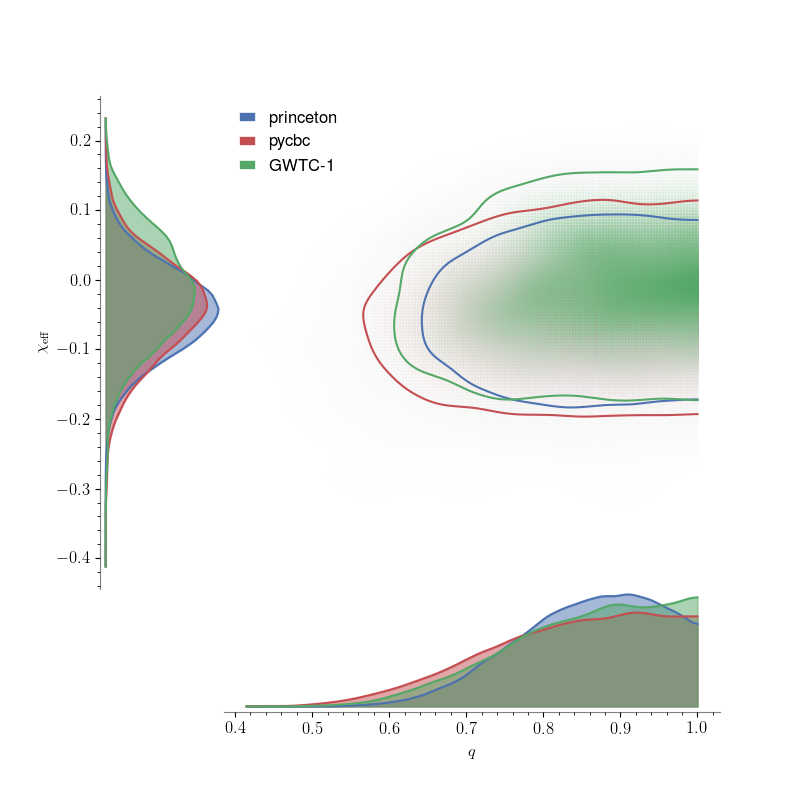
31# Next we generate a `reverse_triangle` plot which compares the mass ratio
32# and effective spin posterior samples
33fig, _, _, _ = data.plot(["mass_ratio", "chi_eff"], type="reverse_triangle", module="gw")
34fig.savefig("comparison_for_GW150914.png")
35fig.close()