Basics of parameter estimation
In this example, we’ll go into some of the basics of parameter estimation and
how they are implemented in bilby.
Firstly, consider a situation where you have discrete data
This is a well studied problem known as linear regression and there already exists many ways to estimate the coefficients (you may already be familiar with a least squares estimator for example).
Here, we will describe a Bayesian approach using nested sampling which might feel
like overkill for this problem. However, it is a useful way to introduce some
of the basic features of bilby before seeing them in more complicated
settings.
The maths
Given the data, the posterior distribution for the model parameters is given by
where the first term on the right-hand-side is the likelihood while the
second is the prior. In the model
Next, we assume that all data points are independent. As such,
When solving problems on a computer, it is often convenient to work with
the log-likelihood. Indeed, a bilby likelihood must have a log_likelihood()
method. For the normal distribution, the log-likelihood for n data points is
Finally, we need to specify a prior. In this case we will use uncorrelated uniform priors
The choice of prior in general should be guided by physical knowledge about the system and not the data in question.
The key point to take away here is that the likelihood and prior are
the inputs to figuring out the posterior. There are many ways to go about
this, we will now show how to do so in bilby. In this case, we explicitly
show how to write the GaussianLikelihood so that one can see how the
maths above gets implemented. For the prior, this is done implicitly by the
naming of the priors.
The code
In the following example, also available under examples/core_examples/linear_regression.py we will step through the process of generating some simulated data, writing a likelihood and prior, and running nested sampling using bilby.
 1#!/usr/bin/env python
 2"""
 3An example of how to use bilby to perform parameter estimation for
 4non-gravitational wave data. In this case, fitting a linear function to
 5data with background Gaussian noise
 6
 7"""
 8import bilby
 9import matplotlib.pyplot as plt
10import numpy as np
11
12# A few simple setup steps
13label = "linear_regression"
14outdir = "outdir"
15bilby.utils.check_directory_exists_and_if_not_mkdir(outdir)
16
17
18# First, we define our "signal model", in this case a simple linear function
19def model(time, m, c):
20    return time * m + c
21
22
23# Now we define the injection parameters which we make simulated data with
24injection_parameters = dict(m=0.5, c=0.2)
25
26# For this example, we'll use standard Gaussian noise
27
28# These lines of code generate the fake data. Note the ** just unpacks the
29# contents of the injection_parameters when calling the model function.
30sampling_frequency = 10
31time_duration = 10
32time = np.arange(0, time_duration, 1 / sampling_frequency)
33N = len(time)
34sigma = np.random.normal(1, 0.01, N)
35data = model(time, **injection_parameters) + np.random.normal(0, sigma, N)
36
37# We quickly plot the data to check it looks sensible
38fig, ax = plt.subplots()
39ax.plot(time, data, "o", label="data")
40ax.plot(time, model(time, **injection_parameters), "--r", label="signal")
41ax.set_xlabel("time")
42ax.set_ylabel("y")
43ax.legend()
44fig.savefig("{}/{}_data.png".format(outdir, label))
45
46# Now lets instantiate a version of our GaussianLikelihood, giving it
47# the time, data and signal model
48likelihood = bilby.likelihood.GaussianLikelihood(time, data, model, sigma)
49
50# From hereon, the syntax is exactly equivalent to other bilby examples
51# We make a prior
52priors = dict()
53priors["m"] = bilby.core.prior.Uniform(0, 5, "m")
54priors["c"] = bilby.core.prior.Uniform(-2, 2, "c")
55
56# And run sampler
57result = bilby.run_sampler(
58    likelihood=likelihood,
59    priors=priors,
60    sampler="dynesty",
61    nlive=250,
62    injection_parameters=injection_parameters,
63    outdir=outdir,
64    label=label,
65)
66
67# Finally plot a corner plot: all outputs are stored in outdir
68result.plot_corner()
Running the script above will make a few images. Firstly, the plot of the data:
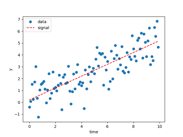
The dashed red line here shows the simulated signal.
Secondly, because we used the plot=True argument in run_sampler we generate a corner plot
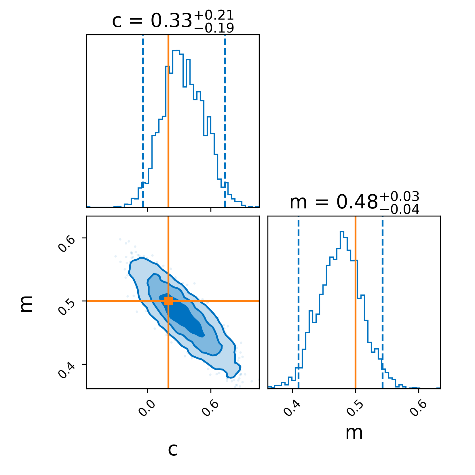
The solid lines indicate the simulated values which are recovered quite easily. Note, you can also make a corner plot with result.plot_corner().
Final thoughts
While this example is somewhat trivial, hopefully you can see how this script can be easily modified to perform parameter estimation for almost any time-domain data where you can model the background noise as Gaussian and write the signal model as a python function (i.e., replacing model).