Dynesty Guide
The Dynesty sampler is just one of the samplers available in bilby, but it is well-used and found to be fast and accurate. Here, we provide a short guide to its implementation. This will not be a complete guide, additional help can be found in the Dynesty documentation.
All of the options discussed herein can be set in the bilby.run_sampler()
call. For example, to set the number of live points to 1000
>>> bilby.run_sampler(likelihood, priors, sampler="dynesty", nlive=1000)
Note
Bilby checks the kwargs input through run_sampler. If you miss-spell a word, you will see a warning “Supplied argument X not an argument of dynesty, removing.”
Bilby-specific implementation details
In Bilby, we have implemented custom stepping methods for use within dynesty.
We have implemented three methods for performing an MCMC evolution to find a
new point from the constrained prior. These can be specified using the
sample argument.
sample="act-walk"(default): with this method, the MCMC evolution is performed until the autocorrelation length of the chain can be accurately determined. Following this guide we run for 50 times the autocorrelation length. This chain is then thinned by a user-specified number of autocorrelation timesnactto yield a cache ofN = 50 / nactpoints. These points are then returned the nextNiterations ofdynesty. With this method,nact=2often gives good results, however, in some cases, a larger value may be required.sample="acceptance-walk": with this method, at each iteration all MCMC chains are set to the same length. The specific length evolves during the run so that the number of accepted steps follows a Poisson distribution with meannacceptduring each chain. This method is well suited to parallelised applications, as each MCMC chain will run for the same amount of time. The value ofnacceptshould be tuned based on the application. For example, one could run a single analysis withsample="act-walk"to estimate a viable number of accepted steps.sample="rwalk": this method is similar to the"acceptance-walk"method, however, the adaptation of the MCMC length happens within the chain. This method is primarily included for historical reasons and was the default method prior toBilby<2. For this application,nactis half the average accepted number of jumps per chain.
You can revert to the original dynesty implementation by specifying
sample="rwalk_dynesty".
There are a number of keyword arguments that influence these sampling methods:
nact/nacceptas described above, this varies based on the method.maxmcmc: the maximum number of walks to use. This naming is chosen for consistency with other codes. Default is 5000. If this limit is reached, a warning will be printed during sampling.proposals: a list of the desired proposals. Each of these proposals can be used with any of the sampling methods described above. The allowed values are
diff: ter Braak + (2006) differential evolution. This is the default forbound="live"andbound="live-multi".
volumetric: sample from an ellipsoid centered on the current point. This is the proposal distribution implemented indynestyand the default for all otherboundoptions. This was the default proposal distribution forBilby<2, however, in many applications it leads to longer autocorrelation times and struggles to explore multi-modal distributions.
Finally, we implement two custom dynesty.sampler.Sampler classes to
facilitate the differential evolution proposal and average acceptance tracking.
bound="live"uses theLivePointSamplerwhich adapts thewalksto averagenacceptaccepted steps when inacceptance-walkmode and passes the current live points to the sample method.bound="live-multi"combines the functionality of"live"with thedynestyimplementedmultimethod for multi-ellipsoidvolumetricsampling. This method is intended when using both thediffandvolumetricproposals.
Understanding the output
Before sampling begins, you will see a message like this
14:06 bilby INFO    : Single likelihood evaluation took 3.273e-03 s
14:06 bilby INFO    : Using sampler Dynesty with kwargs {'nlive': 500, 'bound': 'live', 'sample': 'act-walk', 'periodic': None, 'reflective': None, 'update_interval': 600, 'first_update': None, 'npdim': None, 'rstate': None, 'queue_size': 1, 'pool': None, 'use_pool': None, 'live_points': None, 'logl_args': None, 'logl_kwargs': None, 'ptform_args': None, 'ptform_kwargs': None, 'gradient': None, 'grad_args': None, 'grad_kwargs': None, 'compute_jac': False, 'enlarge': None, 'bootstrap': None, 'walks': 100, 'facc': 0.2, 'slices': None, 'fmove': 0.9, 'max_move': 100, 'update_func': None, 'ncdim': None, 'blob': False, 'save_history': False, 'history_filename': None, 'maxiter': None, 'maxcall': None, 'dlogz': 0.1, 'logl_max': inf, 'n_effective': None, 'add_live': True, 'print_progress': True, 'print_func': <bound method Dynesty._print_func of <bilby.core.sampler.dynesty.Dynesty object at 0x16a3be860>>, 'save_bounds': False, 'checkpoint_file': None, 'checkpoint_every': 60, 'resume': False}
14:06 bilby INFO    : Checkpoint every check_point_delta_t = 600s
14:06 bilby INFO    : Using dynesty version 2.1.0
14:06 bilby INFO    : Using the bilby-implemented rwalk sampling tracking the autocorrelation function and thinning by 2  with maximum length 250000
This tells you that a typical likelihood evaluation takes a few milliseconds.
You can use this to gauge how long the run might take: if a typical likelihood
evaluation takes more than a fraction of a second, it is unlikely your run will
complete in a reasonable amount of time using serial bilby. After this, is a list
of all the kwargs passed in to dynesty. Note, where a None is given,
dynesty will fill in its own defaults. The Bilby specific arguments are printed
on their onw. Then, we get a message about how often checkpointing will be done,
the version of dynesty, and which sample method will be used.
During the sampling, dynesty writes an update of its progress to the terminal (specifally, this is writtent to STDOUT). Here is an example:
1015it [00:08, 138.49it/s, bound:0 nc:2 ncall:2714 eff:37.4% logz-ratio=-67.89+/-0.09 dlogz:181.166>0.10]
From left to right, this gives the number of iterations, the sampling time,
the iterations per second, the bound (while bound=0 dynesty samples
from the unit cube), the number of likelihood calls per sample nc, the
total number of likelihood calls ncall, the sampling efficiency, the
current estimate of the logz-ratio (monotonically increases) and the estimated
remaining log evidence.
If the likelihood calculates the log_noise_evidence, then this output
will give the logz-ratio. If it doesn’t it instead uses just the
unnormalised evidence logz.
The logz-ratio and dlogz gives an estimate of the final
expected evidence. You can compare this to your expectations to help diagnose
problems before completing a run. However, be aware the dlogz does not
monotonically decrease: if a region of large likelihood is subsequently found,
the dlogz will increase.
Diagnostic plots
At each checkpoint, we make a number of plots. Three of these are produced
by dynesty and users should consult the
relevant documentation
for those. (We note that we produce a checkpoint trace with the unit hypercube
samples in addition to the default dynesty plots.)
Finally, we produce a "stats" plot as shown below.
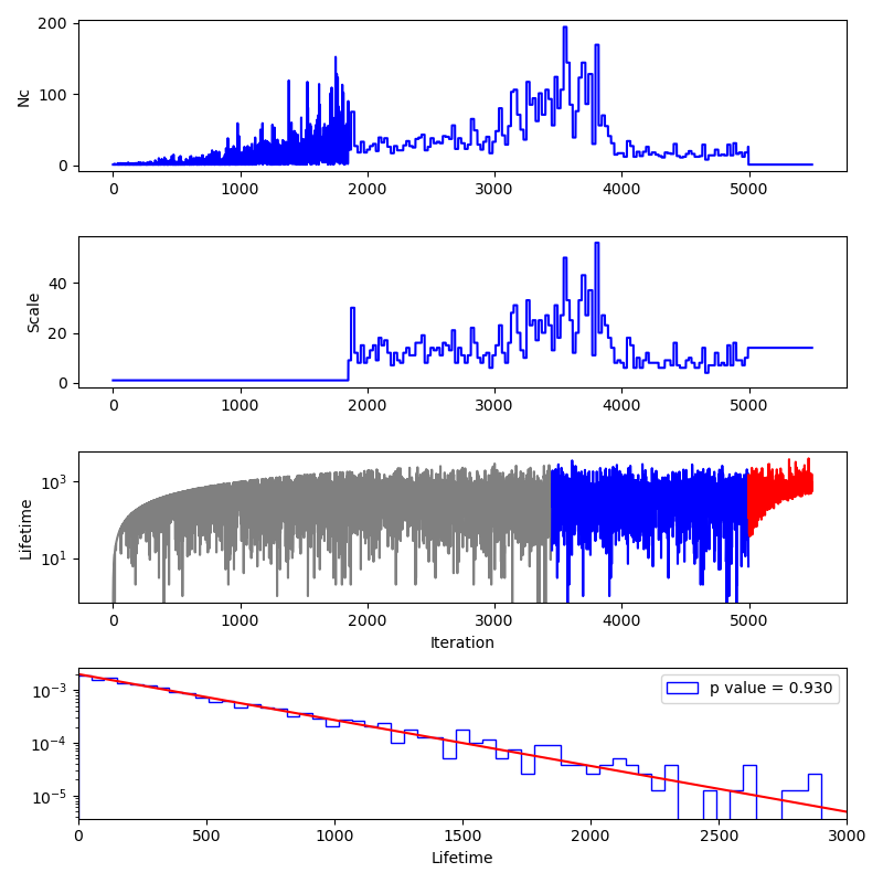
The panels here show:
The number of likelihood evaluations per iteration. The sampling here used the
act-walkmethod and so the flat portions of the curve correspond to points that come from the same MCMC exploration. We can clearly see that in this case, the sampling became much more efficient after 4000 iterations, most likely due to the allowed prior region becoming unimodal at this point.The number of accepted steps per MCMC chain per iteration. Before the MCMC evolution begins, this number is 1 and after the sampling stops, the final value is repeated in the plot.
The number of iterations between a live point being chosen and removed from the ensemble of live points for the point removed at each iteration. This value reaches a stationary distribution after some initial warm-up (shown in grey) and before the final live points are removed (shown in red.)
A histogram of the lifetimes of the blue colored points in the third panel. The red curve shows the expected distribution and the p value compares the lifetimes with the expected distribution.