Prior Distributions with Bilby

Prior distributions are a core component of any Bayesian problem and specifying them in codes can be one of the most confusing elements of a code. The prior modules in Bilby provide functionality for specifying prior distributions in a natural way.

We have a range of predefined types of prior distribution and each kind has methods to:

1. draw samples, prior.sample.

2. calculate the prior probability, prior.prob.

3. rescale samples from a unit cube to the prior distribution, prior.rescale. This is especially useful when using nested samplers as it avoids the need for rejection sampling.

4. Calculate the log prior probability, prior.log_prob.

In addition to the predefined prior distributions there is functionality to specify your own prior, either from a pair of arrays, or from a file.

Each prior distribution can also be given a name and may have a different latex_label for plotting. If no name is provided, the default is None (this should probably by '').

import bilby
import matplotlib.pyplot as plt
import numpy as np

%matplotlib inline

/opt/conda/envs/python310/lib/python3.10/site-packages/pandas/core/computation/expressions.py:21: UserWarning: Pandas requires version '2.8.4' or newer of 'numexpr' (version '2.7.3' currently installed).
  from pandas.core.computation.check import NUMEXPR_INSTALLED

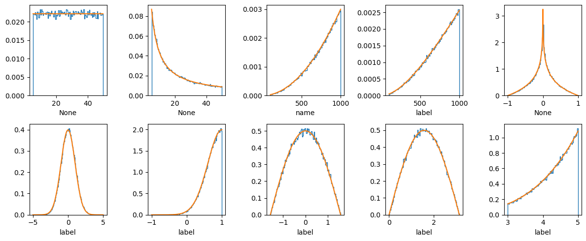
Prior Instantiation

Below we demonstrate instantiating a range of prior distributions.

Note that when a latex_label is not specified, the name is used.

fig = plt.figure(figsize=(12, 5))

priors = [
    bilby.core.prior.Uniform(minimum=5, maximum=50),
    bilby.core.prior.LogUniform(minimum=5, maximum=50),
    bilby.core.prior.PowerLaw(name="name", alpha=2, minimum=100, maximum=1000),
    bilby.gw.prior.UniformComovingVolume(
        name="luminosity_distance", minimum=100, maximum=1000, latex_label="label"
    ),
    bilby.gw.prior.AlignedSpin(),
    bilby.core.prior.Gaussian(name="name", mu=0, sigma=1, latex_label="label"),
    bilby.core.prior.TruncatedGaussian(
        name="name", mu=1, sigma=0.4, minimum=-1, maximum=1, latex_label="label"
    ),
    bilby.core.prior.Cosine(name="name", latex_label="label"),
    bilby.core.prior.Sine(name="name", latex_label="label"),
    bilby.core.prior.Interped(
        name="name",
        xx=np.linspace(0, 10, 1000),
        yy=np.linspace(0, 10, 1000) ** 4,
        minimum=3,
        maximum=5,
        latex_label="label",
    ),
]

for ii, prior in enumerate(priors):
    fig.add_subplot(2, 5, 1 + ii)
    plt.hist(prior.sample(100000), bins=100, histtype="step", density=True)
    if not isinstance(prior, bilby.core.prior.Gaussian):
        plt.plot(
            np.linspace(prior.minimum, prior.maximum, 1000),
            prior.prob(np.linspace(prior.minimum, prior.maximum, 1000)),
        )
    else:
        plt.plot(np.linspace(-5, 5, 1000), prior.prob(np.linspace(-5, 5, 1000)))
    plt.xlabel("{}".format(prior.latex_label))

plt.tight_layout()
plt.show()
plt.close()

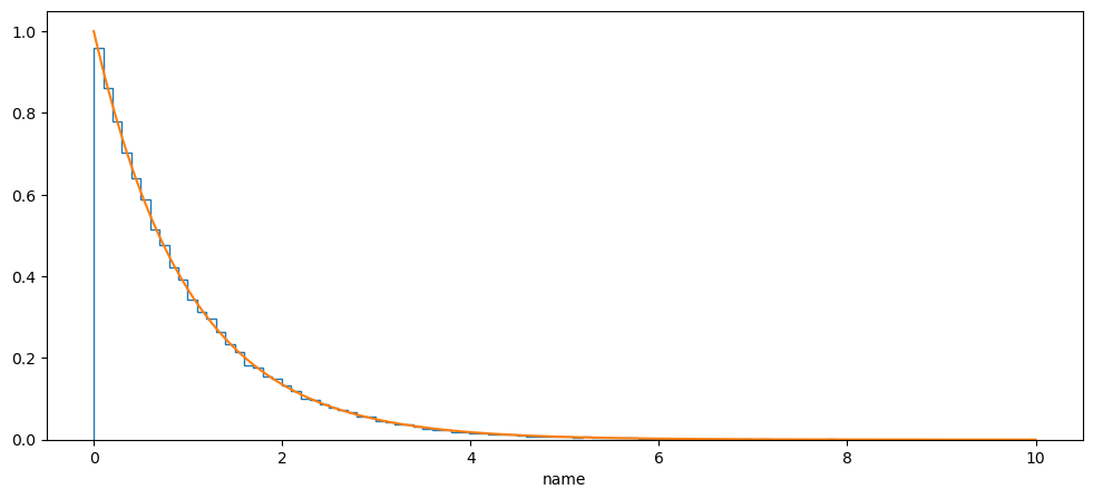
Define an Analytic Prior

Adding a new analytic is achieved as follows.

class Exponential(bilby.core.prior.Prior):
    """Define a new prior class where p(x) ~ exp(alpha * x)"""

    def __init__(self, alpha, minimum, maximum, name=None, latex_label=None):
        super(Exponential, self).__init__(
            name=name, latex_label=latex_label, minimum=minimum, maximum=maximum
        )
        self.alpha = alpha

    def rescale(self, val):
        return (
            np.log(
                (np.exp(self.alpha * self.maximum) - np.exp(self.alpha * self.minimum))
                * val
                + np.exp(self.alpha * self.minimum)
            )
            / self.alpha
        )

    def prob(self, val):
        in_prior = (val >= self.minimum) & (val <= self.maximum)
        return (
            self.alpha
            * np.exp(self.alpha * val)
            / (np.exp(self.alpha * self.maximum) - np.exp(self.alpha * self.minimum))
            * in_prior
        )

prior = Exponential(name="name", alpha=-1, minimum=0, maximum=10)

plt.figure(figsize=(12, 5))
plt.hist(prior.sample(100000), bins=100, histtype="step", density=True)
plt.plot(
    np.linspace(prior.minimum, prior.maximum, 1000),
    prior.prob(np.linspace(prior.minimum, prior.maximum, 1000)),
)
plt.xlabel("{}".format(prior.latex_label))
plt.show()
plt.close()