Compare samplers

In this notebook, we’ll compare the different samplers implemented in Bilby on a simple linear regression problem.

This is not an exhaustive set of the implemented samplers, nor of the settings available for each sampler.

Setup

import bilby
import numpy as np
import matplotlib.pyplot as plt

%matplotlib inline

/opt/conda/envs/python310/lib/python3.10/site-packages/pandas/core/computation/expressions.py:21: UserWarning: Pandas requires version '2.8.4' or newer of 'numexpr' (version '2.7.3' currently installed).
  from pandas.core.computation.check import NUMEXPR_INSTALLED

label = "linear_regression"
outdir = "outdir"
bilby.utils.check_directory_exists_and_if_not_mkdir(outdir)

Define our model

Here our model is a simple linear fit to some quantity \(y = m x + c\).

def model(x, m, c):
    return x * m + c

Simulate data

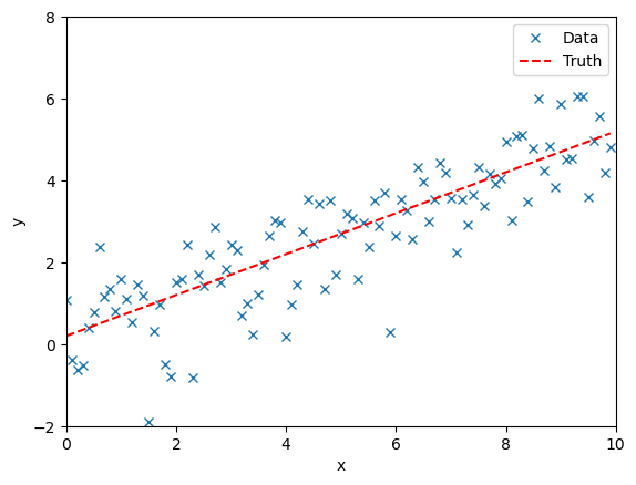
We simulate observational data. We assume some uncertainty in the observations and so perturb the observations from the truth.

injection_parameters = dict(m=0.5, c=0.2)

sampling_frequency = 10
time_duration = 10
time = np.arange(0, time_duration, 1 / sampling_frequency)
N = len(time)
sigma = np.random.normal(1, 0.01, N)
data = model(time, **injection_parameters) + np.random.normal(0, sigma, N)

fig, ax = plt.subplots()
ax.plot(time, data, "x", label="Data")
ax.plot(time, model(time, **injection_parameters), "--r", label="Truth")
ax.set_xlim(0, 10)
ax.set_ylim(-2, 8)
ax.set_xlabel("x")
ax.set_ylabel("y")
ax.legend()
plt.show()
plt.close()

Define the likelihood and prior

For any Bayesian calculation we need a likelihood and a prior.

In this case, we take a GausianLikelihood as we assume the uncertainty on the data is normally distributed.

For both of our parameters we take uniform priors.

likelihood = bilby.likelihood.GaussianLikelihood(time, data, model, sigma)

priors = bilby.core.prior.PriorDict()
priors["m"] = bilby.core.prior.Uniform(0, 5, "m")
priors["c"] = bilby.core.prior.Uniform(-2, 2, "c")

Run the samplers and compare the inferred posteriors

We’ll use four of the implemented samplers.

For each one we specify a set of parameters.

Bilby/the underlying samplers produce quite a lot of output while the samplers are running so we will suppress as many of these as possible.

After running the analysis, we print a final summary for each of the samplers.

samplers = dict(
    bilby_mcmc=dict(
        nsamples=1000,
        L1steps=20,
        ntemps=10,
        printdt=10,
    ),
    dynesty=dict(npoints=500, sample="acceptance-walk", naccept=20),
    pymultinest=dict(nlive=500),
    nestle=dict(nlive=500),
    emcee=dict(nwalkers=20, iterations=500),
    ptemcee=dict(ntemps=10, nwalkers=20, nsamples=1000),
)

results = dict()

bilby.core.utils.logger.setLevel("ERROR")

for sampler in samplers:
    result = bilby.core.sampler.run_sampler(
        likelihood,
        priors=priors,
        sampler=sampler,
        label=sampler,
        resume=False,
        clean=True,
        verbose=False,
        **samplers[sampler]
    )
    results[sampler] = result

 *****************************************************
 MultiNest v3.10
 Copyright Farhan Feroz & Mike Hobson
 Release Jul 2015

 no. of live points =  500
 dimensionality =    2
 *****************************************************

  analysing data from /tmp/tmpb7zr1wrl/.txt ln(ev)=  -146.69688830340621      +/-  0.10858889035030130
 Total Likelihood Evaluations:         5488
 Sampling finished. Exiting MultiNest

print("=" * 40)
for sampler in results:
    print(sampler)
    print("=" * 40)
    print(results[sampler])
    print("=" * 40)

========================================
bilby_mcmc
========================================
nsamples: 2605
ln_noise_evidence:    nan
ln_evidence: -143.726 +/-  0.028
ln_bayes_factor:    nan +/-  0.028

========================================
dynesty
========================================
nsamples: 1341
ln_noise_evidence:    nan
ln_evidence: -146.578 +/-  0.135
ln_bayes_factor:    nan +/-  0.135

========================================
pymultinest
========================================
nsamples: 1760
ln_noise_evidence:    nan
ln_evidence: -146.697 +/-  0.109
ln_bayes_factor:    nan +/-  0.109

========================================
nestle
========================================
nsamples: 4424
ln_noise_evidence:    nan
ln_evidence: -146.806 +/-  0.109
ln_bayes_factor:    nan +/-  0.109

========================================
emcee
========================================
nsamples: 8620
ln_noise_evidence:    nan
ln_evidence:    nan +/-    nan
ln_bayes_factor:    nan +/-    nan

========================================
ptemcee
========================================
nsamples: 1020
ln_noise_evidence:    nan
ln_evidence: -150.976 +/- 19.113
ln_bayes_factor:    nan +/- 19.113

========================================

Make comparison plots

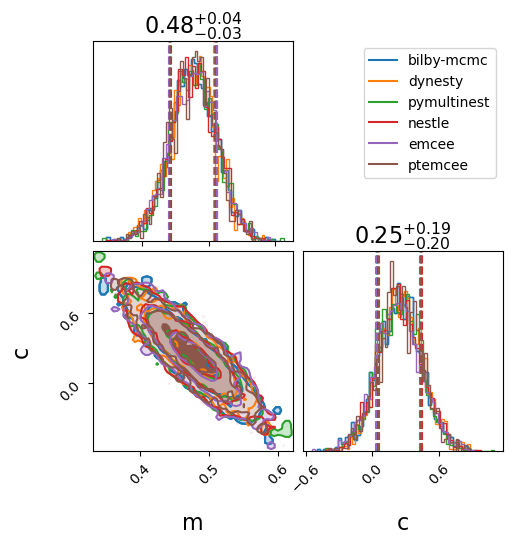
We will make two standard comparison plots.

In the first we plot the one- and two-dimensional marginal posterior distributions in a “corner” plot.

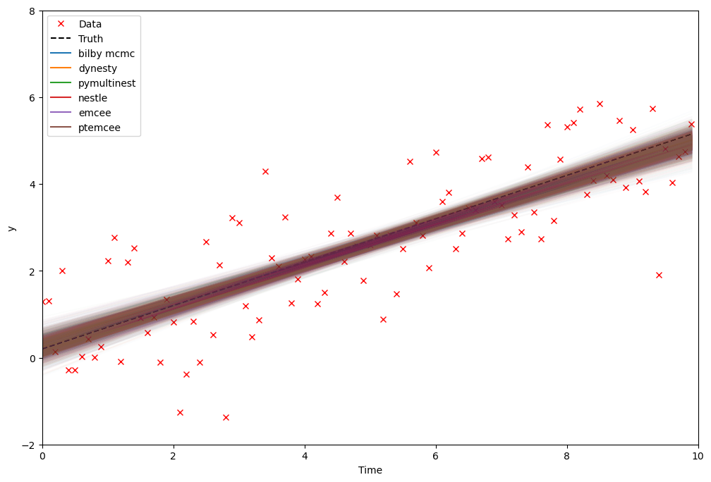
In the second, we show the inferred model that we are fitting along with the uncertainty by taking random draws from the posterior distribution. This kind of posterior predicitive plot is useful to identify model misspecification.

_ = bilby.core.result.plot_multiple(
    list(results.values()), labels=list(results.keys()), save=False
)
plt.show()
plt.close()

fig, ax = plt.subplots(figsize=(12, 8))
ax.plot(time, data, "x", label="Data", color="r")
ax.plot(
    time, model(time, **injection_parameters), linestyle="--", color="k", label="Truth"
)

for jj, sampler in enumerate(samplers):
    result = results[sampler]
    samples = result.posterior[result.search_parameter_keys].sample(500)
    for ii in range(len(samples)):
        parameters = dict(samples.iloc[ii])
        plt.plot(time, model(time, **parameters), color=f"C{jj}", alpha=0.01)
    plt.axhline(-10, color=f"C{jj}", label=sampler.replace("_", " "))
ax.set_xlim(0, 10)
ax.set_ylim(-2, 8)
ax.set_xlabel("Time")
ax.set_ylabel("y")
ax.legend(loc="upper left")
plt.show()
plt.close()