Compact binary coalescence parameter estimation
In this example, we demonstrate how to generate simulated data for a binary black hole coalescence observed by the two LIGO interferometers at Hanford and Livingston for all parameters in the IMRPhenomPv2 waveform model.
The code will take around 15 hours to run.
For testing, you may prefer to run the 4-parameter CBC tutorial.
  1#!/usr/bin/env python
  2"""
  3Tutorial to demonstrate running parameter estimation on a full 15 parameter
  4space for an injected cbc signal. This is the standard injection analysis script
  5one can modify for the study of injected CBC events.
  6
  7This will take many hours to run.
  8"""
  9import bilby
 10import numpy as np
 11
 12# Set the duration and sampling frequency of the data segment that we're
 13# going to inject the signal into
 14duration = 4.0
 15sampling_frequency = 1024.0
 16
 17# Specify the output directory and the name of the simulation.
 18outdir = "outdir"
 19label = "full_15_parameters"
 20bilby.core.utils.setup_logger(outdir=outdir, label=label)
 21
 22# Set up a random seed for result reproducibility.  This is optional!
 23np.random.seed(88170235)
 24
 25# We are going to inject a binary black hole waveform.  We first establish a
 26# dictionary of parameters that includes all of the different waveform
 27# parameters, including masses of the two black holes (mass_1, mass_2),
 28# spins of both black holes (a, tilt, phi), etc.
 29injection_parameters = dict(
 30    mass_1=36.0,
 31    mass_2=29.0,
 32    a_1=0.4,
 33    a_2=0.3,
 34    tilt_1=0.5,
 35    tilt_2=1.0,
 36    phi_12=1.7,
 37    phi_jl=0.3,
 38    luminosity_distance=2000.0,
 39    theta_jn=0.4,
 40    psi=2.659,
 41    phase=1.3,
 42    geocent_time=1126259642.413,
 43    ra=1.375,
 44    dec=-1.2108,
 45)
 46
 47# Fixed arguments passed into the source model
 48waveform_arguments = dict(
 49    waveform_approximant="IMRPhenomXPHM",
 50    reference_frequency=50.0,
 51    minimum_frequency=20.0,
 52)
 53
 54# Create the waveform_generator using a LAL BinaryBlackHole source function
 55# the generator will convert all the parameters
 56waveform_generator = bilby.gw.WaveformGenerator(
 57    duration=duration,
 58    sampling_frequency=sampling_frequency,
 59    frequency_domain_source_model=bilby.gw.source.lal_binary_black_hole,
 60    parameter_conversion=bilby.gw.conversion.convert_to_lal_binary_black_hole_parameters,
 61    waveform_arguments=waveform_arguments,
 62)
 63
 64# Set up interferometers.  In this case we'll use two interferometers
 65# (LIGO-Hanford (H1), LIGO-Livingston (L1). These default to their design
 66# sensitivity
 67ifos = bilby.gw.detector.InterferometerList(["H1", "L1"])
 68ifos.set_strain_data_from_power_spectral_densities(
 69    sampling_frequency=sampling_frequency,
 70    duration=duration,
 71    start_time=injection_parameters["geocent_time"] - 2,
 72)
 73
 74ifos.inject_signal(
 75    waveform_generator=waveform_generator, parameters=injection_parameters
 76)
 77
 78# For this analysis, we implement the standard BBH priors defined, except for
 79# the definition of the time prior, which is defined as uniform about the
 80# injected value.
 81# We change the mass boundaries to be more targeted for the source we
 82# injected.
 83# We define priors in the time at the Hanford interferometer and two
 84# parameters (zenith, azimuth) defining the sky position wrt the two
 85# interferometers.
 86priors = bilby.gw.prior.BBHPriorDict()
 87
 88time_delay = ifos[0].time_delay_from_geocenter(
 89    injection_parameters["ra"],
 90    injection_parameters["dec"],
 91    injection_parameters["geocent_time"],
 92)
 93priors["H1_time"] = bilby.core.prior.Uniform(
 94    minimum=injection_parameters["geocent_time"] + time_delay - 0.1,
 95    maximum=injection_parameters["geocent_time"] + time_delay + 0.1,
 96    name="H1_time",
 97    latex_label="$t_H$",
 98    unit="$s$",
 99)
100del priors["ra"], priors["dec"]
101priors["zenith"] = bilby.core.prior.Sine(latex_label="$\\kappa$")
102priors["azimuth"] = bilby.core.prior.Uniform(
103    minimum=0, maximum=2 * np.pi, latex_label="$\\epsilon$", boundary="periodic"
104)
105
106# Initialise the likelihood by passing in the interferometer data (ifos) and
107# the waveoform generator, as well the priors.
108# The explicit distance marginalization is turned on to improve
109# convergence, and the posterior is recovered by the conversion function.
110likelihood = bilby.gw.GravitationalWaveTransient(
111    interferometers=ifos,
112    waveform_generator=waveform_generator,
113    priors=priors,
114    distance_marginalization=True,
115    phase_marginalization=False,
116    time_marginalization=False,
117    reference_frame="H1L1",
118    time_reference="H1",
119)
120
121# Run sampler. In this case we're going to use the `dynesty` sampler
122# Note that the `walks`, `nact`, and `maxmcmc` parameter are specified
123# to ensure sufficient convergence of the analysis.
124# We set `npool=4` to parallelize the analysis over four cores.
125# The conversion function will determine the distance posterior in post processing
126result = bilby.run_sampler(
127    likelihood=likelihood,
128    priors=priors,
129    sampler="dynesty",
130    nlive=1000,
131    walks=20,
132    nact=50,
133    maxmcmc=2000,
134    npool=4,
135    injection_parameters=injection_parameters,
136    outdir=outdir,
137    label=label,
138    conversion_function=bilby.gw.conversion.generate_all_bbh_parameters,
139    result_class=bilby.gw.result.CBCResult,
140)
141
142# Plot the inferred waveform superposed on the actual data.
143result.plot_waveform_posterior(n_samples=1000)
144
145# Make a corner plot.
146result.plot_corner()
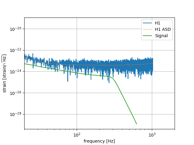
Running this script will generate data then perform parameter estimation. In doing all of this, it prints information about the matched-filter SNRs in each detector (saved to the log-file). Moreover, it generates a plot for each detector showing the data, amplitude spectral density (ASD) and the signal; here is an example for the Hanford detector:
Finally, after running the parameter estimation. It generates a corner plot:
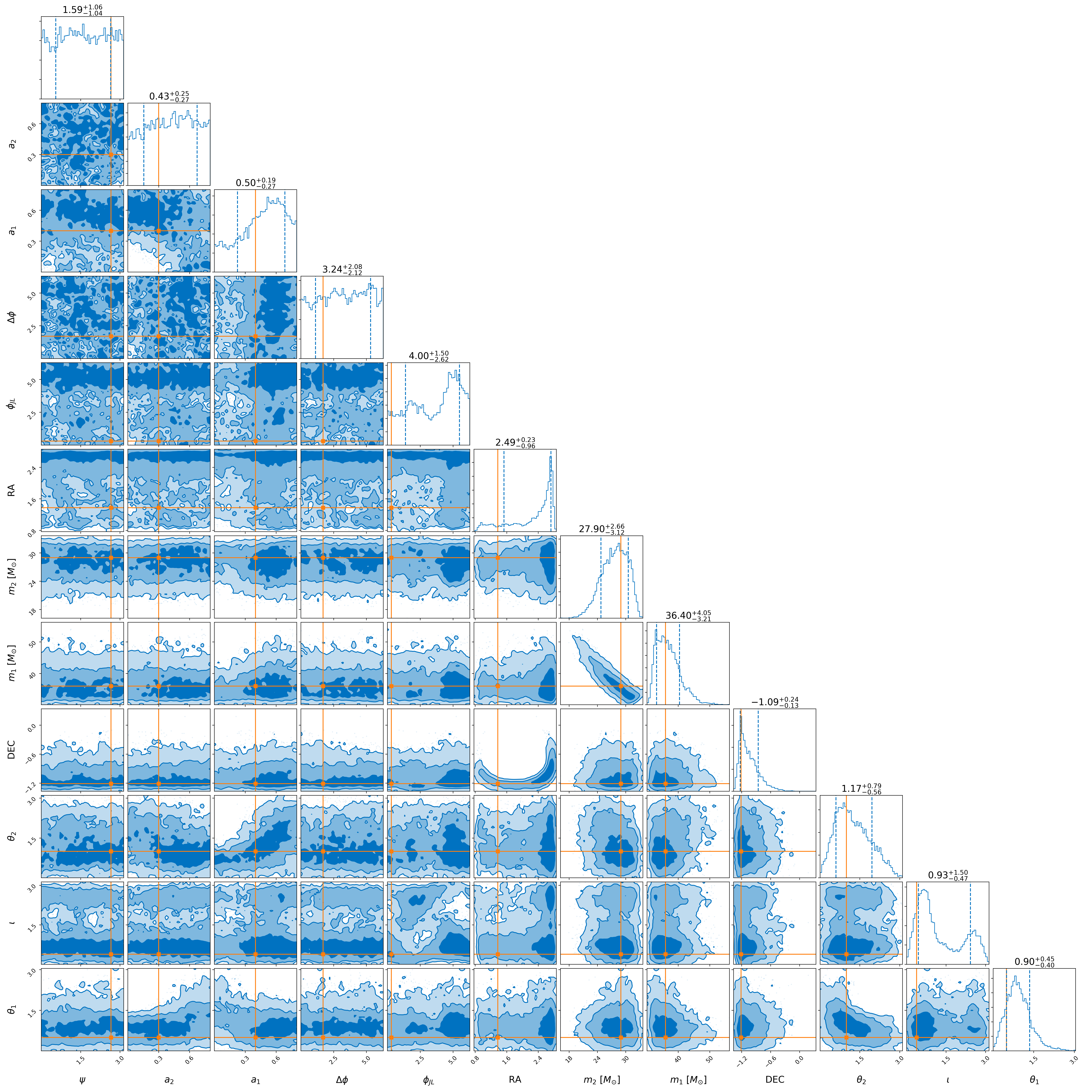
The solid lines indicate the injection parameters.